Tutorial

This tutorial introduces the main reasons to use Abapy and explains how to do so. In order to follow the tutorial, following components are required:

• Abaqus
• Python (2.5 or above) and its modules Numpy, Scipy, Matplotlib, SQLAlchemy.

Introduction

Indentation testing is used widely as an example in this tutorial but everything can be transposed easily to any other problem. Let’s start with an existing axisymmetric conical indentation simulations defined in the following INP file: indentation_axi.inp. The model includes following features:

• Axisymmetric solids.
• Conical rigid indenter.
• Von Mises elastic-plastic sample.
• Frictionless contact.
• Non linear geometry effects.

The simulation can be launched directly using the command-line:

abaqus job=indentation-axi

Note

The INP file can also be imported in Abaqus/CAE through file/import/model and then by chosing .inp. Then create a job and launch it.

The simulation is normaly very fast because the meshes are rather coarse. When it is completed, you can open the resulting ODB file using abaqus viewer to have a look at it. Then, then you can start to go deeper into the ODB structure. Use a terminal or DOS shell to launch the following command:

abaqus viewer -noGUI

You are now in the Python interface of Abaqus/Viewer.

Note

The are several ways to access Python in Abaqus. abaqus python is the standard way, it is faster since it doesn’t require a licence token. However, you will often need packages that are not available in abaqus python, then you will have to use abaqus viewer -noGUI or abaqus cae -noGUI which both allow access to everything that is available in Abaqus/viewer and Abaqus/CAE.

Now that you have access to Python inside Abaqus, you can open the odb file using:

>>> from odbAccess import openOdb
>>> odb = openOdb('indentation_axi.odb')

Then you can have a look at the structure of the odb object mainly using the print and dir commands.

>>> dir(odb)
['AcousticInfiniteSection', 'AcousticInterfaceSection', 'ArbitraryProfile', 'BeamSection', 'BoxProfile', 'CircularProfile', 'CohesiveSection', 'CompositeShellSection', 'CompositeSolidSection', 'ConnectorSection', 'DiscretePart', 'GasketSection', 'GeneralStiffnessSection', 'GeneralizedProfile', 'GeometryShellSection', 'HexagonalProfile', 'HomogeneousShellSection', 'HomogeneousSolidSection', 'IProfile', 'LProfile', 'Material', 'MembraneSection', 'PEGSection', 'Part', 'PipeProfile', 'RectangularProfile', 'Section', 'SectionCategory', 'Step', 'SurfaceSection', 'TProfile', 'TrapezoidalProfile', 'TrussSection', 'UserXYData', '__class__', '__cmp__', '__delattr__', '__doc__', '__getattribute__', '__hash__', '__init__', '__new__', '__reduce__', '__reduce_ex__', '__repr__', '__setattr__', '__str__', 'analysisTitle', 'close', 'closed', 'customData', 'description', 'diagnosticData', 'getFrame', 'isReadOnly', 'jobData', 'materials', 'name', 'parts', 'path', 'profiles', 'rootAssembly', 'save', 'sectionCategories', 'sections', 'sectorDefinition', 'steps', 'update', 'userData']
>>> # OK let's have a look inside jobData
>>> print odb.jobData
({'analysisCode': ABAQUS_STANDARD, 'creationTime': 'Mon Apr 29 15:44:54 CEST 2013', 'machineName': '', 'modificationTime': 'Mon Apr 29 15:44:55 CEST 2013', 'name': '/home/lcharleux/Documents/Programmation/Python/Modules/abapy/doc/example_code/tutorial/workdir/indentation_axi.odb', 'precision': SINGLE_PRECISION, 'productAddOns': (), 'version': 'Abaqus/Standard 6.9-EF1'})
>>> print odb.diagnosticData
({'analysisErrors': 'OdbSequenceAnalysisError object', 'analysisWarnings': 'OdbSequenceAnalysisWarning object', 'isXplDoublePrecision': False, 'jobStatus': JOB_STATUS_COMPLETED_SUCCESSFULLY, 'jobTime': 'OdbJobTime object', 'numDomains': 1, 'numberOfAnalysisErrors': 0, 'numberOfAnalysisWarnings': 1, 'numberOfSteps': 2, 'numericalProblemSummary': 'OdbNumericalProblemSummary object', 'steps': 'OdbSequenceDiagnosticStep object'})
>>> print odb.diagnosticData.jobStatus
JOB_STATUS_COMPLETED_SUCCESSFULLY
>>> # Now we know that the simulation was successful
>>> # Let's now have a look to history outputs
>>> print odb.steps
{'LOADING': 'OdbStep object', 'UNLOADING': 'OdbStep object'}
>>> print odb.steps['LOADING']
({'acousticMass': -1.0, 'acousticMassCenter': (), 'description': '', 'domain': TIME, 'eliminatedNodalDofs': 'NodalDofsArray object', 'frames': 'OdbFrameArray object', 'historyRegions': 'Repository object', 'inertiaAboutCenter': (), 'inertiaAboutOrigin': (), 'loadCases': 'Repository object', 'mass': -1.0, 'massCenter': (), 'name': 'LOADING', 'nlgeom': True, 'number': 1, 'previousStepName': 'Initial', 'procedure': '*STATIC', 'retainedEigenModes': (), 'retainedNodalDofs': 'NodalDofsArray object', 'timePeriod': 1.0, 'totalTime': 0.0})
>>> print odb.steps['LOADING'].frames[-1]
({'cyclicModeNumber': None, 'description': 'Increment     20: Step Time =    1.000', 'domain': TIME, 'fieldOutputs': 'Repository object', 'frameId': 20, 'frameValue': 1.0, 'frequency': None, 'incrementNumber': 20, 'isImaginary': False, 'loadCase': None, 'mode': None})
>>> print odb.steps['LOADING'].historyRegions['Assembly ASSEMBLY']
({'description': 'Output at assembly ASSEMBLY', 'historyOutputs': 'Repository object', 'loadCase': None, 'name': 'Assembly ASSEMBLY', 'point': 'HistoryPoint object', 'position': WHOLE_MODEL})
>>> # And then to field outputs
>>> print odb.steps['LOADING'].frames[-1].fieldOutputs['U'].values[0]
({'baseElementType': '', 'conjugateData': None, 'conjugateDataDouble': 'unknown', 'data': array([-2.51322398980847e-06, -0.333516657352448], 'd'), 'dataDouble': 'unknown', 'elementLabel': None, 'face': None, 'instance': 'OdbInstance object', 'integrationPoint': None, 'inv3': None, 'localCoordSystem': None, 'localCoordSystemDouble': 'unknown', 'magnitude': 0.333516657352448, 'maxInPlanePrincipal': None, 'maxPrincipal': None, 'midPrincipal': None, 'minInPlanePrincipal': None, 'minPrincipal': None, 'mises': None, 'nodeLabel': 1, 'outOfPlanePrincipal': None, 'position': NODAL, 'precision': SINGLE_PRECISION, 'press': None, 'sectionPoint': None, 'tresca': None, 'type': VECTOR})

At this point, you must understand that you can find back every single input as well as every output in through Python. The question is now how to do it painlessly. Abapy was originaly made to solve this problem even if it can perform many other tasks like preprocessing and data management.

First example

Let’s now try to get back the load vs. disp curve and plot it using Abapy. First, we have to emphasize that Abaqus Python is not the best place to run any calculation or to plot things. There are many reasons for that among which:

• Abaqus uses old versions of Python, sometimes 5 years behind the current stable versions.
• It can be painful or even impossible to install packages on Abaqus/Python, for example on servers where you don’t have admin rights.

This point is essential to understand how Abapy is built. Every function or class that can be used inside Abaqus/Python does not rely on third party packages like Numpy, even if it could be of great utility. On the other hand, classes that work on Abaqus/Python can have methods that use numpy locally because they are not intended to be used inside Abaqus. Then, the post processing with Abapy is intended to be done in two steps:

• Step 1: grabbing raw data inside Abaqus/Python and save it, mainly using serialization built-in module Pickle.
• Step 2: Processing raw data inside a standard Python on which third party modules are available.

Now that we clarified this point, we will work with both Abaqus/Python and Python. The second one will progressively take more importance and become our main concern. We can make a first script that will be executed inside Abaqus/Python. It aims to find where to find the indenter displacement of the force applied on it.

# ABAQUS/PYTHON POST PROCESSING SCRIPT
# Run using abaqus python / abaqus viewer -noGUI / abaqus cae -noGUI

# Packages (Abaqus, Abapy and built-in only here)
from odbAccess import openOdb
from abapy.misc import dump
from abapy.postproc import GetHistoryOutputByKey as gho

# Setting up some pathes
workdir = 'workdir'
name = 'indentation_axi'

# Opening the Odb File
odb = openOdb(workdir + '/' + name + '.odb')

# Finding back the position of the reference node of the indenter. Its number is stored inside a node set named REF_NODE.
ref_node_label = odb.rootAssembly.instances['I_INDENTER'].nodeSets['REF_NODE'].nodes[0].label

# Getting back the reaction forces along Y (RF2) and displacements along Y (U2) where they are recorded.
RF2 = gho(odb, 'RF2')
U2  = gho(odb, 'U2')

# Packing data
data = {'ref_node_label': ref_node_label, 'RF2':RF2, 'U2':U2}

# Dumping data
dump(data, workdir + '/' + name + '.pckl')

# Closing Odb
odb.close()

Dowload link: first_example_abq.py

Then, we can make a second script that is made to work in regular Python

# PYTHON POST PROCESSING SCRIPT
# Run using python

# Packages
from abapy.misc import load
import matplotlib.pyplot as plt
import numpy as np

# Setting up some pathes
workdir = 'workdir'
name = 'indentation_axi'

# Getting back raw data
data = load(workdir + '/' + name + '.pckl')

# Post processing
ref_node_label = data['ref_node_label']
force_hist = -data['RF2']['Node I_INDENTER.{0}'.format(ref_node_label)]
disp_hist = -data['U2']['Node I_INDENTER.{0}'.format(ref_node_label)]

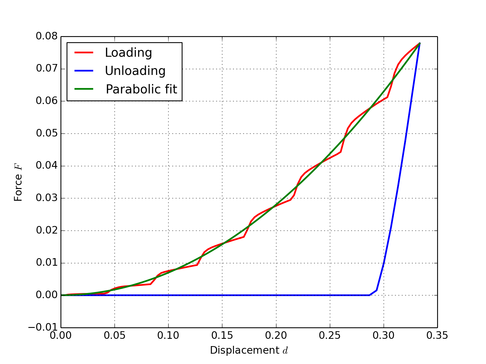
time, force_l = force_hist[0,1].plotable() # Getting back force  during loading
time, disp_l = disp_hist[0,1].plotable()   # Getting backdisplacement during loading
time, force_u = force_hist[2].plotable() # Getting back force  during unloading
time, disp_u = disp_hist[2].plotable()   # Getting backdisplacement during unloading

# Dimensional analysis (E. Buckingham. Physical review, 4, 1914.) shows that the loading curve must be parabolic, let's build a parabolic fit


C_factor = (force_hist[1] / disp_hist[1]**2).average()
disp_fit = np.array(disp_hist[0,1].toArray()[1])
force_fit = C_factor * disp_fit**2


plt.figure()
plt.clf()
plt.plot(disp_l, force_l, 'r-', linewidth = 2., label = 'Loading')
plt.plot(disp_u, force_u, 'b-', linewidth = 2., label = 'Unloading')
plt.plot(disp_fit, force_fit, 'g-', linewidth = 2., label = 'Parabolic fit')
plt.xlabel('Displacement $d$')
plt.ylabel('Force $F$')
plt.grid()
plt.legend(loc = 'upper left')
plt.show()

(Source code, png, hires.png, pdf)

The loading curve is very noisy because the mesh is coarse. Anyway, the loading phase is theoretically parabolic and so, it can be averaged and give a quite good result even if looks ugly.

Fancier example

Now we want to do fancier things like wrapping all the Abaqus/Python part inside the regular Python part in order to change the problem into a simple function or method evaluation. On a more mechanical point of view, we want to be able to compute the loading prefactor C for any material parameters usable in the von Mises elastic plastic law. We create 2 files:

# FANCIER_EXAMPLE: computing the loading prefactor of the indentation load vs. disp curve.
# Run using python

# Packages
from abapy.misc import load
import matplotlib.pyplot as plt
import numpy as np

     


def compute_C(E = 1. , nu = 0.3, sy = 0.01, abqlauncher = '/opt/Abaqus/6.9/Commands/abaqus', workdir = 'workdir', name = 'indentation_axi_fancier', frames = 50):
  '''
  Computes the load prefactor C using Abaqus.
  
  Inputs:
  * E: sample's Young modulus.
  * nu: samples's Poisson's ratio
  * sy: sample's yield stress (von Mises yield criterion).
  * abqlauncher: absolute path to abaqus launcher.
  * wordir: path to working directory, can be relative.
  * name: name of simulation files.
  * frames: number of frames per step, increase if the simulation does not complete.
  
  Returns:
  * Load prefactor C (float)
  '''
  import time, subprocess, os
  t0 = time.time() # Starting time recording
  path = workdir + '/' + name
  # Reading the INP target file
  f = open('indentation_axi_target.inp', 'r')
  inp = f.read()
  f.close()
  # Replace the targets in the file
  inp = inp.replace('#E', '{0}'.format(E))
  inp = inp.replace('#NU', '{0}'.format(nu))
  inp = inp.replace('#SY', '{0}'.format(sy))
  inp = inp.replace('#FRAME', '{0}'.format(1./frames))
  # Creating a new inp file
  f = open(path  + '.inp', 'w')
  f.write(inp)
  f.close()
  print 'Created INP file: {0}.inp'.format(path)
  # Then we run the simulation
  print 'Running simulation in Abaqus'
  p = subprocess.Popen( '{0} job={1} input={1}.inp interactive ask_delete=OFF'.format(abqlauncher, name), cwd = workdir, shell=True, stdout = subprocess.PIPE)
  trash = p.communicate()
  
  # Now we test run the post processing script
  print 'Post processing the simulation in Abaqus/Python'
  p = subprocess.Popen( [abqlauncher,  'viewer', 'noGUI=fancier_example_abq.py'], cwd = '.',stdout = subprocess.PIPE )
  trash = p.communicate()
  # Getting back raw data
  data = load(workdir + '/' + name + '.pckl')
  # Post processing
  print 'Post processing the simulation in Python'
  if data['completed']:
    ref_node_label = data['ref_node_label']
    force_hist = -data['RF2']['Node I_INDENTER.{0}'.format(ref_node_label)]
    disp_hist = -data['U2']['Node I_INDENTER.{0}'.format(ref_node_label)]
    trash, force_l = force_hist[0,1].plotable() # Getting back force  during loading
    trash, disp_l = disp_hist[0,1].plotable()   # Getting backdisplacement during loading
    trash, force_u = force_hist[2].plotable() # Getting back force  during unloading
    trash, disp_u = disp_hist[2].plotable()   # Getting backdisplacement during unloading
    C_factor = (force_hist[1] / disp_hist[1]**2).average()
    
  else:
    print 'Simulation aborted, probably because frame number is to low'
    C_factor = None  
  t1 = time.time()
  print 'Time used: {0:.2e} s'.format(t1-t0)
  return C_factor
  
# Setting up some pathes
workdir = 'workdir'
name = 'indentation_axi_fancier'
abqlauncher = '/opt/Abaqus/6.9/Commands/abaqus'

# Setting material parameters
E = 1.
nu = 0.3
sy = 0.01
frames = 50

# Testing it all
C = compute_C(E = E, nu = nu, sy = sy, frames = frames)
print 'C = {0}'.format(C)

Dowload link: fancier_example.py

# ABAQUS/PYTHON POST PROCESSING SCRIPT
# Run using abaqus python / abaqus viewer -noGUI / abaqus cae -noGUI

# Packages (Abaqus, Abapy and built-in only here)
from odbAccess import openOdb
from abapy.misc import dump
from abapy.postproc import GetHistoryOutputByKey as gho
from abaqusConstants import JOB_STATUS_COMPLETED_SUCCESSFULLY


# Setting up some pathes
workdir = 'workdir'
name = 'indentation_axi_fancier'

# Opening the Odb File
odb = openOdb(workdir + '/' + name + '.odb')

# Testing job status
data = {}
status = odb.diagnosticData.jobStatus
if status == JOB_STATUS_COMPLETED_SUCCESSFULLY:
  data['completed'] = True
  # Finding back the position of the reference node of the indenter. Its number is stored inside a node set named REF_NODE.
  ref_node_label = odb.rootAssembly.instances['I_INDENTER'].nodeSets['REF_NODE'].nodes[0].label

  # Getting back the reaction forces along Y (RF2) and displacements along Y (U2) where they are recorded.
  RF2 = gho(odb, 'RF2')
  U2  = gho(odb, 'U2')

  # Packing data
  data['ref_node_label'] = ref_node_label
  data['RF2'] = RF2 
  data['U2']  = U2

  
else:
  data['completed'] = False
# Dumping data
dump(data, workdir + '/' + name + '.pckl')
# Closing Odb
odb.close()

Dowload link: fancier_example_abq.py

Then, executing fancier_example.py gives:

>>> execfile('fancier_example.py')
Created INP file: workdir/indentation_axi_fancier.inp
Running simulation in Abaqus
Abaqus License Manager checked out the following licenses:
Abaqus/Standard checked out 5 tokens.
<55 out of 60 licenses remain available>.
Abaqus License Manager checked out the following licenses:
Abaqus/Standard checked out 5 tokens.
<55 out of 60 licenses remain available>.
Post processing the simulation in Abaqus/Python
Abaqus License Manager checked out the following license(s):
"cae" release 6.9 from epua-e172.univ-savoie.fr
<5 out of 6 licenses remain available>.
Post processing the simulation in Python
Time used: 2.93e+01 s
C = 0.6993227005

Now you know how how to control the simulation through regular Python but important things are still missing. For example:

• The coarse mesh limits the accuracy of the simulation, a parametric mesh allowing to adjust speed and precision freely would be welcomed.
• What if you need more that the single load prefactor ? A class having many important outputs instead of a function could be nice.
• Simulations take time and it’s always frustrating to do them two times, data persistence could of great use here.

All this can be addressed using Abapy with other third party packages like Numpy, Scipy, Matplotlib and SQLAlchemy. The advanced example provides details explanations on this point.