Materials
Material definitions.
Elastic materials
-
class
abapy.materials.Elastic(labels='mat', E=1.0, nu=0.3, dtf='d')[source]¶ Represents an istotrop linear elastic material used for FEM simulations
Parameters: - E (float, list, array.array) – Young’s modulus.
- nu (float, list, array.array) – Poisson’s ratio.
Note
All inputs must have the same length or an exception will be raised.
Elastic-plastic materials
-
class
abapy.materials.VonMises(labels='mat', E=1.0, nu=0.3, sy=0.01, dtf='d')[source]¶ Represents von Mises materials used for FEM simulations
Parameters: - E (float, list, array.array) – Young’s modulus.
- nu (float, list, array.array) – Poisson’s ratio.
- sy (float, list, array.array) – Yield stress.
Note
All inputs must have the same length or an exception will be raised.
>>> from abapy.materials import VonMises
>>> m = VonMises(labels='myMaterial',E=1,nu=0.45, sy=0.01)
>>> print m.dump2inp()
...
-
class
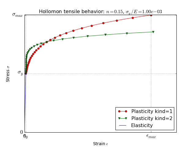
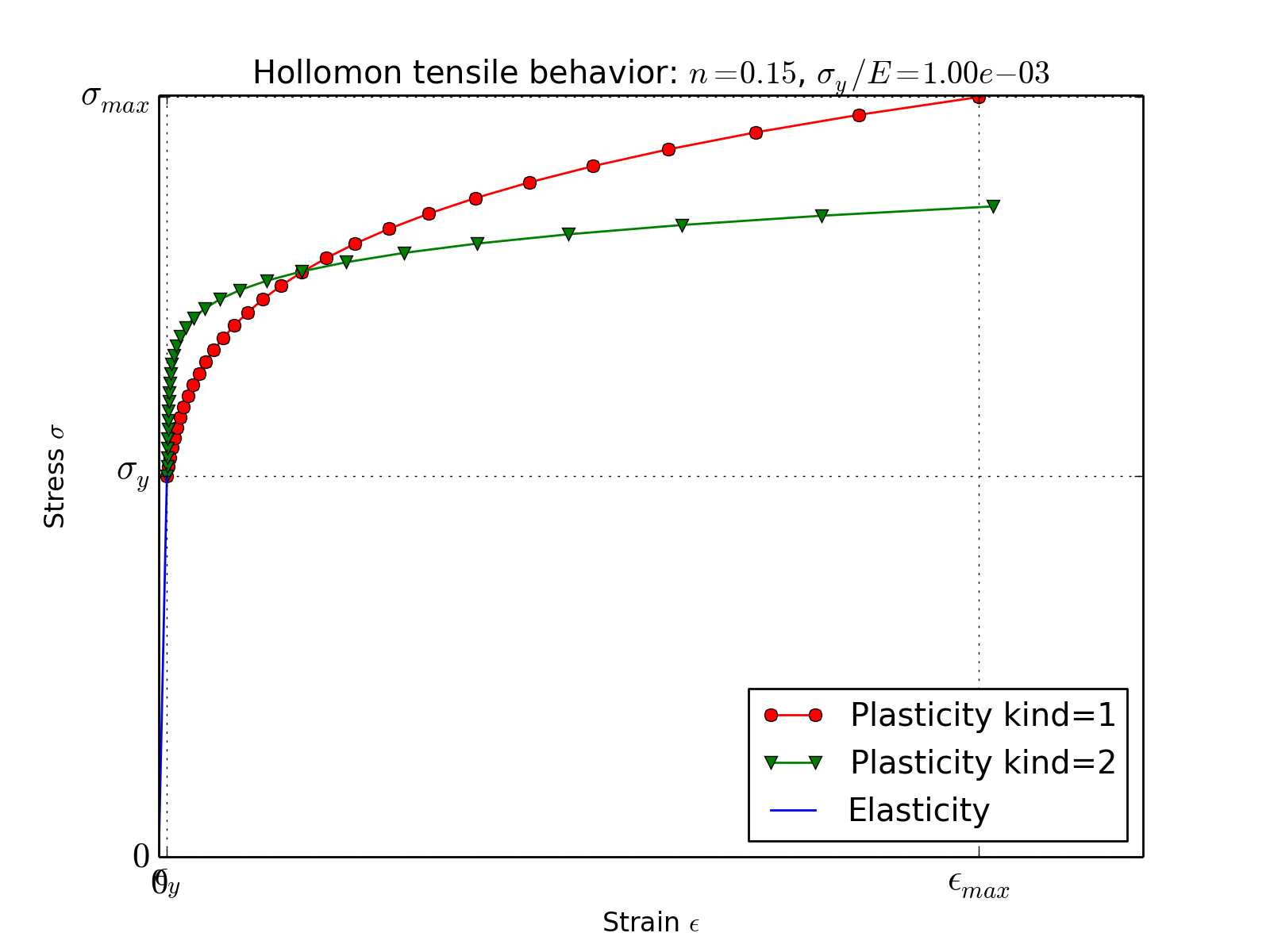
abapy.materials.Hollomon(labels='mat', E=1.0, nu=0.3, sy=0.01, n=0.2, kind=1, dtf='d')[source]¶ Represents von Hollom materials (i. e. power law haderning and von mises yield criterion) used for FEM simulations.
Parameters: - E (float, list, array.array) – Young’s modulus.
- nu (float, list, array.array) – Poisson’s ratio.
- sy (float, list, array.array) – Yield stress.
- n – hardening exponent
- kind (int) – kind of equation to be used (see below). Default is 1.
Note
All inputs must have the same length or an exception will be raised.
Several sets of equations are refered to as Hollomon stress-strain law. In all cases, we the strain decomposition
 is used and the elastic part is described by
  . Only the plastic parts (i. e.
  ) differ:
- kind 1:

- kind 2:

from abapy.materials import Hollomon
import matplotlib.pyplot as plt

E = 1.       # Young's modulus
sy = 0.001     # Yield stress
n = 0.15    # Hardening exponent
nu = 0.3
eps_max = .1 # maximum strain to be computed
N = 30      # Number of points to be computed (30 is a low value useful for graphical reasons, in real simulations, 100 is a better value).
mat1 = Hollomon(labels = 'my_material', E=E, nu=nu, sy=sy, n=n)
table1 = mat1.get_table(0, N=N, eps_max=eps_max)
eps1 = table1[:,0]
sigma1 = table1[:,1]
sigma_max1 = max(sigma1)

mat2 = Hollomon(labels = 'my_material', E=E, nu=nu, sy=sy, n=n, kind = 2)
table2 = mat2.get_table(0, N=N, eps_max=eps_max)
eps2 = table2[:,0]
sigma2 = table2[:,1]
sigma_max2 = max(sigma2)


plt.figure()
plt.clf()
plt.title('Hollomon tensile behavior: $n = {0:.2f}$, $\sigma_y / E = {1:.2e}$'.format(n, sy/E))
plt.xlabel('Strain $\epsilon$')
plt.ylabel('Stress $\sigma$')
plt.plot(eps1, sigma1, 'or-', label = 'Plasticity kind=1')
plt.plot(eps2, sigma2, 'vg-', label = 'Plasticity kind=2')
plt.plot([0., sy / E], [0., sy], 'b-', label = 'Elasticity')
plt.xticks([0., sy/E, eps_max], ['$0$', '$\epsilon_y$', '$\epsilon_{max}$'], fontsize = 16.)
plt.yticks([0., sy, sigma_max1], ['$0$', '$\sigma_y$', '$\sigma_{max}$'], fontsize = 16.)
plt.grid()
plt.legend(loc = "lower right")
plt.show()
(Source code, png, hires.png, pdf)
-
dump2inp(eps_max=10.0, N=100)[source]¶ Returns materials in INP format suitable with abaqus input files.
Parameters: - eps_max (float) – maximum strain to be computed.
- N (int) – number of points to be computed.
Return type: string
-
get_table(position=0, eps_max=10.0, N=100)[source]¶ Returns the tabular data corresponding to the tensile stress strain law using log spacing. :param position: indice of the concerned material (default is 0). :type position: int :param eps_max: maximum strain to be computed. If kind is 1, eps_max is the total strain, if kind is 2, eps_max is the plastic strain. :type eps_max: float :param N: number of points to be computed. :type N: int :rtype:
numpy.array
-
class
abapy.materials.DruckerPrager(labels='mat', E=1.0, nu=0.3, sy=0.01, beta=10.0, psi=None, k=1.0, dtf='d')[source]¶ Represents Drucker-Prager materials used for FEM simulations
Parameters: - E (float, list, array.array) – Young’s modulus.
- nu (float, list, array.array) – Poisson’s ratio.
- sy (float, list, array.array) – Compressive yield stress.
- beta (float, list, array.array) – Friction angle in degrees.
- psi (float, list, array.array or None) – Dilatation angle in degress. If psi = beta, the plastic flow is associated. If psi = None, the associated flow is automatically be chosen.
- k (float, list, array.array) – tension vs. compression asymmetry. For k = 1., not asymmetry, for k=0.778 maximum possible asymmetry.
Note
All inputs must have the same length or an exception will be raised....
-
class
abapy.materials.Bilinear(labels='mat', E=1.0, nu=0.3, Ssat=1000.0, n=100.0, sy=100.0, dtf='d')[source]¶ Represents von Mises materials used for FEM simulations
Parameters: - E (float, list, array.array) – Young’s modulus.
- nu (float, list, array.array) – Poisson’s ratio.
- Ssat (float, list, array.array) – Saturation stress.
- n (float, list, array.array) – Slope of the first linear plastic law
- Sy (float, list, array.array) – Stress at zero plastic strain
Note
All inputs must have the same length or an exception will be raised.