Mesh
Mesh processing tools.
Nodes
-
class
abapy.mesh.Nodes(labels=[], x=[], y=[], z=[], sets={}, dtf='f', dti='I')[source]¶ Manages nodes for finite element modeling pre/postprocessing and further graphical representations.
Parameters: - labels (list of int > 0) – list of node labels.
- x (list floats) – x coordinate of nodes.
- y (list floats) – y coordinate of nodes.
- z (list floats) – z coordinate of nodes.
- sets (dict with str keys and where values are list of ints > 0.) – node sets
- dti ('I' or 'H') – int data type in array.array
- dtf ('f' or 'd') – float data type in array.array
>>> from abapy.mesh import Nodes
>>> labels = [1,2]
>>> x = [0., 1.]
>>> y = [0., 2.]
>>> z = [0., 0.]
>>> sets = {'mySet': [1,2]}
>>> nodes = Nodes(labels = labels, x = x, y = y, z = z, sets = sets)
>>> nodes
<Nodes class instance: 2 nodes>
>>> print nodes
Nodes class instance:
Nodes:
Label x       y       z
1     0.0     0.0     0.0
2     1.0     2.0     0.0
Sets:
Label Nodes
myset 1,2
>>> from abapy.mesh import Nodes
>>> labels = range(1,11) # 10 nodes
>>> x = labels
>>> y = labels
>>> z = [0. for i in x]
>>> nodes = Nodes(labels=labels, x=x, y=y, z=z)
>>> nodes.add_set('myset',[4,5,6,9]) # A set
>>> print nodes
Nodes class instance:
Nodes:
Label x       y       z
1     1.0     1.0     0.0
2     2.0     2.0     0.0
3     3.0     3.0     0.0
4     4.0     4.0     0.0
5     5.0     5.0     0.0
6     6.0     6.0     0.0
7     7.0     7.0     0.0
8     8.0     8.0     0.0
9     9.0     9.0     0.0
10    10.0    10.0    0.0
Sets:
Label Nodes
myset 4,5,6,9
>>> print nodes[5] # requesting node 5
Nodes class instance:
Nodes:
Label x       y       z
5     5.0     5.0     0.0
Sets:
Label Nodes
myset 5
>>> print nodes[5,4,10]  # requesting nodes 5, 4 and 10. Note that output has ordered nodes and kept sets.
Nodes class instance:
Nodes:
Label x       y       z
4     4.0     4.0     0.0
5     5.0     5.0     0.0
10    10.0    10.0    0.0
Sets:
Label Nodes
myset 5,4
>>> print nodes['myset'] # requesting nodes using set key
Nodes class instance:
Nodes:
Label x       y       z
4     4.0     4.0     0.0
5     5.0     5.0     0.0
6     6.0     6.0     0.0
9     9.0     9.0     0.0
Sets:
Label Nodes
myset 4,5,6,9
>>> print nodes['myset',10] # mixed request: nodes in myset AND node 10.
Nodes class instance:
Nodes:
Label x       y       z
4     4.0     4.0     0.0
5     5.0     5.0     0.0
6     6.0     6.0     0.0
9     9.0     9.0     0.0
10    10.0    10.0    0.0
Sets:
Label Nodes
myset 4,5,6,9
>>> print nodes[1:9:2] # slice
Nodes class instance:
Nodes:
Label x       y       z
1     1.0     1.0     0.0
3     3.0     3.0     0.0
5     5.0     5.0     0.0
7     7.0     7.0     0.0
Sets:
Label Nodes
myset 5
Add/remove/get data
-
Nodes.add_node(label=None, x=0.0, y=0.0, z=0.0, toset=None)[source]¶ Adds one node to Nodes instance.
Parameters: - label – If None, label is automatically chosen to be the highest existing label + 1 (default: None). If label (and susequently node) already exists, a warning is printed and the node is not added and sets that could be created ar not created.
- x (float) – x coordinate of node.
- y (float) – y coordinate of node.
- z (float) – z coordinate of node.
- tosets – set(s) to which the node should be added. If a set does not exist, it is created. If None, the node is not added to any set.
>>> from abapy.mesh import Nodes
>>> nodes = Nodes()
>>> nodes.add_node(label = 10, x = 0., y = 0., z = 0., toset = 'firstSet')
>>> print nodes
Nodes class instance:
Nodes:
Label       x       y       z
10  0.0     0.0     0.0
Sets:
Label       Nodes
firstset    10
>>> nodes.add_node(x = 0., y = 0., z = 0., toset = ['firstSet', 'secondSet'])
>>> print nodes
Nodes class instance:
Nodes:
Label       x       y       z
10  0.0     0.0     0.0
11  0.0     0.0     0.0
Sets:
Label       Nodes
firstset    10,11
secondset   11
-
Nodes.drop_node(label)[source]¶ Removes one node to Nodes instance. The node is also removed from sets, if a set happens to be empty, it is also removed.
Parameters: label (int > 0) – node be removed’s label. >>> from abapy.mesh import Nodes >>> nodes = labels = [1,2] >>> x = [0., 1.] >>> y = [0., 2.] >>> z = [0., 0.] >>> sets = {'mySet': [2]} >>> nodes = Nodes(labels = labels, x = x, y = y, z = z, sets = sets) >>> print nodes Nodes class instance: Nodes: Label x y z 1 0.0 0.0 0.0 2 1.0 2.0 0.0 Sets: Label Nodes myset 2 >>> nodes.drop_node(2) >>> print nodes Nodes class instance: Nodes: Label x y z 1 0.0 0.0 0.0 Sets: Label Nodes
-
Nodes.add_set(label, nodes)[source]¶ Adds a node set to the Nodes instance or appends nodes to existing node sets.
Parameters: - label (string) – set to be added’s label.
- nodes (int or list of ints) – nodes to be added in the set.
Note
set labels are always lower case in this class to be case insensitive. This way to proceed is coherent with Abaqus.
>>> from abapy.mesh import Nodes
>>> nodes = Nodes()
>>> labels = [1,2]
>>> x = [0., 1.]
>>> y = [0., 2.]
>>> z = [0., 0.]
>>> sets = {'mySet': 2}
>>> nodes = Nodes(labels = labels, x = x, y = y, z = z, sets = sets)
>>> print nodes
Nodes class instance:
Nodes:
Label       x       y       z
1   0.0     0.0     0.0
2   1.0     2.0     0.0
Sets:
Label       Nodes
myset       2
>>> nodes.add_set('MYSET',1)
>>> print nodes
Nodes class instance:
Nodes:
Label       x       y       z
1   0.0     0.0     0.0
2   1.0     2.0     0.0
Sets:
Label       Nodes
myset       2,1
>>> nodes.add_set('MyNeWseT',[1,2])
>>> print nodes
Nodes class instance:
Nodes:
Label       x       y       z
1   0.0     0.0     0.0
2   1.0     2.0     0.0
Sets:
Label       Nodes
myset       2,1
mynewset    1,2
-
Nodes.add_set_by_func(name, func)[source]¶ Creates a node set using a function of x, y, z and labels (given as
numpy.array). Must get back a boolean array of the same size.Parameters: - name (string) – set label.
- func (function) – function of x, y ,z and labels
>>> mesh.nodes.add_set_by_func('setlabel', lambda x, y, z, labels: x == 0.)
-
Nodes.drop_set(label)[source]¶ Drops a set without removing elements and nodes.
Parameters: label (string) – label of the to be removed. >>> from abapy.mesh import Nodes >>> labels = range(1,11) >>> x = labels >>> y = labels >>> z = [0. for i in x] >>> nodes = Nodes(labels=labels, x=x, y=y, z=z) >>> nodes.add_set('myset',[4,5,6,9]) >>> print nodes Nodes class instance: Nodes: Label x y z 1 1.0 1.0 0.0 2 2.0 2.0 0.0 3 3.0 3.0 0.0 4 4.0 4.0 0.0 5 5.0 5.0 0.0 6 6.0 6.0 0.0 7 7.0 7.0 0.0 8 8.0 8.0 0.0 9 9.0 9.0 0.0 10 10.0 10.0 0.0 Sets: Label Nodes myset 4,5,6,9 >>> nodes.drop_set('someSet') Info: sets someset does not exist and cannot be dropped. >>> nodes.drop_set('MYSET') >>> print nodes Nodes class instance: Nodes: Label x y z 1 1.0 1.0 0.0 2 2.0 2.0 0.0 3 3.0 3.0 0.0 4 4.0 4.0 0.0 5 5.0 5.0 0.0 6 6.0 6.0 0.0 7 7.0 7.0 0.0 8 8.0 8.0 0.0 9 9.0 9.0 0.0 10 10.0 10.0 0.0 Sets: Label Nodes
Modifications
-
Nodes.translate(x=0.0, y=0.0, z=0.0)[source]¶ Translates all the nodes.
Parameters: - x (float) – translation along x value.
- y (float) – translation along y value.
- z (float) – translation along z value.
>>> from abapy.mesh import Nodes
>>> nodes = Nodes()
>>> labels = [1,2]
>>> x = [0., 1.]
>>> y = [0., 2.]
>>> z = [0., 0.]
>>> sets = {'mySet': 2}
>>> nodes = Nodes(labels = labels, x = x, y = y, z = z, sets = sets)
>>> nodes.translate(x = 1., y=0., z = -4.)
>>> print nodes
Nodes class instance:
Nodes:
Label       x       y       z
1   1.0     0.0     -4.0
2   2.0     2.0     -4.0
Sets:
Label       Nodes
myset       2
-
Nodes.apply_displacement(disp)[source]¶ Applies a displacement field to the nodes.
Parameters: disp ( VectorFieldOutputinstance) – displacement field.from abapy.mesh import Mesh, Nodes, RegularQuadMesh import matplotlib.pyplot as plt from numpy import cos, sin, pi from copy import copy def function(x, y, z, labels): r0 = 1. theta = 2 * pi * x r = y + r0 ux = -x + r * cos(theta) uy = -y + r * sin(theta) uz = 0. * z return ux, uy, uz N1, N2 = 100, 25 l1, l2 = .75, 1. Ncolor = 20 mesh = RegularQuadMesh(N1 = N1, N2 = N2, l1 = l1, l2 = l2) vectorField = mesh.nodes.eval_vectorFunction(function) mesh.nodes.apply_displacement(vectorField) field = vectorField.get_coord(2) # we chose to plot coordinate 2 field2 = vectorField.get_coord(2) # we chose to plot coordinate 2 x,y,z = mesh.get_edges() # Mesh edges X,Y,Z,tri = mesh.dump2triplot() xb,yb,zb = mesh.get_border() # mesh borders xe, ye, ze = mesh.get_edges() fig = plt.figure(figsize=(10,10)) fig.gca().set_aspect('equal') plt.axis('off') plt.plot(xb,yb,'k-', linewidth = 2.) plt.plot(xe, ye,'k-', linewidth = .5) plt.tricontour(X,Y,tri,field.data, Ncolor, colors = 'black') color = plt.tricontourf(X,Y,tri,field.data, Ncolor) plt.colorbar(color) plt.show()
-
Nodes.closest_node(label)[source]¶ Finds the closest node of an existing node.
Parameters: label (int > 0) – node label to be used. Return type: label (int > 0) and distance (float) of the closest node.
-
Nodes.replace_node(old, new)[source]¶ Replaces a node of given label (old) by another existing node (new).
-
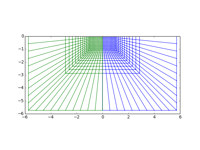
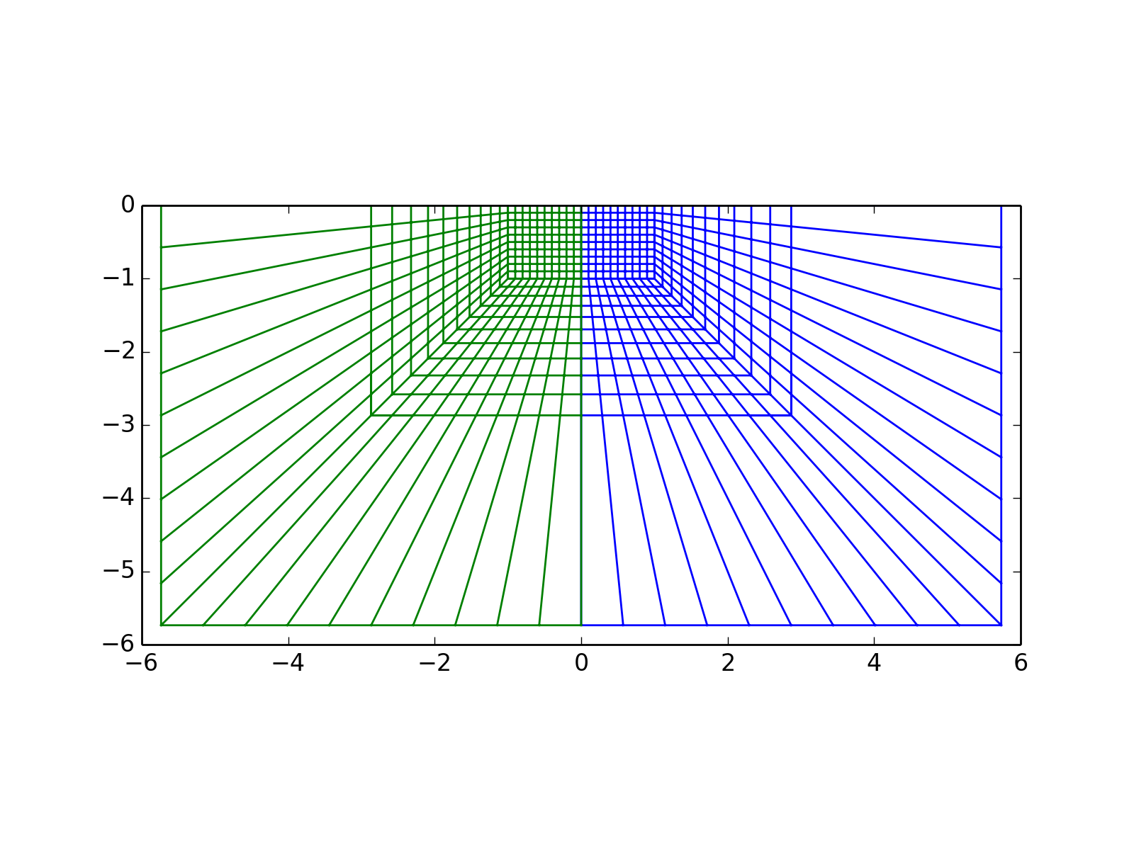
Mesh.apply_reflection(point=(0.0, 0.0, 0.0), normal=(1.0, 0.0, 0.0))[source]¶ Applies a reflection symmetry to the mesh instance. The reflection plane is defined by a point and a normal direction.
Parameters: - point (tuple or list containing 3 floats) – coordinates of a point of the reflection plane.
- normal (tuple or list containing 3 floats) – normal vector to the reflection plane
Return type: Meshinstance..note: This method can lead to coherence problems with surfaces, this problem will be addressed in the future. Surfaces are removed by this operation untill this problem is solved.
from abapy.mesh import RegularQuadMesh
from abapy.indentation import ParamInfiniteMesh
import matplotlib.pyplot as plt

point  = (0., 0., 0.)
normal = (1., 0., 0.)
m0 = ParamInfiniteMesh()
x0, y0, z0 = m0.get_edges()
m1 = m0.apply_reflection(normal = normal, point = point)
x1, y1, z1 = m1.get_edges()
plt.plot(x0, y0)
plt.plot(x1, y1)
plt.gca().set_aspect('equal')
plt.show()
(Source code, png, hires.png, pdf)
Export
-
Nodes.dump2inp()[source]¶ Dumps Nodes instance to Abaqus INP format.
Return type: string >>> from abapy.mesh import Nodes >>> nodes = Nodes() >>> labels = [1,2] >>> x = [0., 1.] >>> y = [0., 2.] >>> z = [0., 0.] >>> sets = {'mySet': 2} >>> nodes = Nodes(labels = labels, x = x, y = y, z = z, sets = sets) >>> out = nodes.dump2inp()
Tools
-
Nodes.eval_function(function)[source]¶ Evals a function at each node and returns a
FieldOutputinstance.Parameters: function (function) – a function with arguments x, y and z (float numpy.arrayscontaining nodes coordinates) and labels (intnumpy.array). Field should not depend on labels but on some vicious problem, it could be useful. The function should return 1 array.Return type: `FieldOutput`instance.from abapy.mesh import Mesh, Nodes, RegularQuadMesh import matplotlib.pyplot as plt from numpy import cos, pi def function(x, y, z, labels): r = (x**2 + y**2)**.5 return cos(2*pi*x)*cos(2*pi*y)/(r+1.) N1, N2 = 100, 25 l1, l2 = 4., 1. Ncolor = 20 mesh = RegularQuadMesh(N1 = N1, N2 = N2, l1 = l1, l2 = l2) field = mesh.nodes.eval_function(function) x,y,z = mesh.get_edges() # Mesh edges X,Y,Z,tri = mesh.dump2triplot() xb,yb,zb = mesh.get_border() fig = plt.figure(figsize=(16,4)) fig.gca().set_aspect('equal') fig.frameon = True plt.plot(xb,yb,'k-', linewidth = 2.) plt.xticks([0,l1],['$0$', '$l_1$'], fontsize = 15.) plt.yticks([0,l2],['$0$', '$l_2$'], fontsize = 15.) plt.tricontourf(X,Y,tri,field.data, Ncolor) plt.tricontour(X,Y,tri,field.data, Ncolor, colors = 'black') plt.show()
-
Nodes.eval_vectorFunction(function)[source]¶ Evals a vector function at each node and returns a
VectorFieldOutputinstance.Parameters: function (function) – a vector function with arguments x, y and z (float numpy.arrayscontaining nodes coordinates) and labels (intnumpy.array). Field should not depend on labels but on some vicious problem, it could be useful. The function should return 3 arrays.Return type: `FieldOutput`instance.from abapy.mesh import Mesh, Nodes, RegularQuadMesh import matplotlib.pyplot as plt from numpy import cos, sin, pi def function(x, y, z, labels): r0 = 1. theta = 2 * pi * x r = y + r0 ux = -x + r * cos(theta) uy = -y + r * sin(theta) uz = 0. * z return ux, uy, uz N1, N2 = 100, 25 l1, l2 = 1., 1. Ncolor = 20 mesh = RegularQuadMesh(N1 = N1, N2 = N2, l1 = l1, l2 = l2) vectorField = mesh.nodes.eval_vectorFunction(function) field = vectorField.get_coord(1) # we chose to plot coordinate 1 field2 = vectorField.get_coord(2) # we chose to plot coordinate 1 field3 = vectorField.norm() # we chose to plot norm fig = plt.figure(figsize=(16,4)) ax = fig.add_subplot(131) ax2 = fig.add_subplot(132) ax3 = fig.add_subplot(133) ax.set_aspect('equal') ax2.set_aspect('equal') ax3.set_aspect('equal') ax.set_xticks([]) ax.set_yticks([]) ax2.set_xticks([]) ax2.set_yticks([]) ax3.set_xticks([]) ax3.set_yticks([]) ax.set_frame_on(False) ax2.set_frame_on(False) ax3.set_frame_on(False) ax.set_title(r'$V_1$') ax2.set_title(r'$V_2$') ax3.set_title(r'$\sqrt{\vec{V}^2}$') ax3.set_title(r'$||\vec{V}||$') x,y,z = mesh.get_edges() # Mesh edges xt,yt,zt = mesh.convert2tri3().get_edges() # Triangular mesh edges xb,yb,zb = mesh.get_border() X,Y,Z,tri = mesh.dump2triplot() ax.plot(xb,yb,'k-', linewidth = 2.) ax.tricontourf(X,Y,tri,field.data, Ncolor) ax.tricontour(X,Y,tri,field.data, Ncolor, colors = 'black') ax2.plot(xb,yb,'k-', linewidth = 2.) ax2.tricontourf(X,Y,tri,field2.data, Ncolor) ax2.tricontour(X,Y,tri,field2.data, Ncolor, colors = 'black') ax3.plot(xb,yb,'k-', linewidth = 2.) ax3.tricontourf(X,Y,tri,field3.data, Ncolor) ax3.tricontour(X,Y,tri,field3.data, Ncolor, colors = 'black') ax.set_xlim([-.1*l1,1.1*l1]) ax.set_ylim([-.1*l2,1.1*l2]) ax2.set_xlim([-.1*l1,1.1*l1]) ax2.set_ylim([-.1*l2,1.1*l2]) ax3.set_xlim([-.1*l1,1.1*l1]) ax3.set_ylim([-.1*l2,1.1*l2]) plt.show()
-
Nodes.eval_tensorFunction(function)[source]¶ Evaluates a tensor function at each node and returns a
tensorFieldOutputinstance.Parameters: function (function) – a tensor function with arguments x, y and z (float numpy.arrayscontaining nodes coordinates) and labels (intnumpy.array). Field should not depend on labels but on some vicious problem, it could be useful. The function should return 6 arrays corresponding to indices ordered as follows: 11, 22, 33, 12, 13, 23.Return type: `FieldOutput`instance.from abapy.mesh import Mesh, Nodes, RegularQuadMesh import matplotlib.pyplot as plt from numpy import cos, sin, pi, linspace def boussinesq(r, z, theta, labels): ''' Stress solution of the Boussinesq point loading of semi infinite elastic half space for a force F = 1. and nu = 0.3 ''' from math import pi from numpy import zeros_like nu = 0.3 rho = (r**2 + z**2)**.5 s_rr = -1./(2. * pi * rho**2) * ( (-3. * r**2 * z)/(rho**3) + (1.-2. * nu)*rho / (rho + z) ) #s_rr = 1./(2.*pi) *( (1-2*nu) * ( r**-2 -z / (rho * r**2)) - 3 * z * r**2 / rho**5 ) s_zz = 3. / (2. *pi ) * z**3 / rho**5 s_tt = -( 1. - 2. * nu) / (2. * pi * rho**2 ) * ( z/rho - rho / (rho + z) ) #s_tt = ( 1. - 2. * nu) / (2. * pi ) * ( 1. / r**2 -z/( rho * r**2) -z / rho**3 ) s_rz = -3./ (2. * pi) * r * z**2 / rho **5 s_rt = zeros_like(r) s_zt = zeros_like(r) return s_rr, s_zz, s_tt, s_rz, s_rt, s_zt return ux, uy, uz N1, N2 = 50, 50 l1, l2 = 1., 1. Ncolor = 200 levels = linspace(0., 10., 20) mesh = RegularQuadMesh(N1 = N1, N2 = N2, l1 = l1, l2 = l2) # Finding the node located at x = y =0.: nodes = mesh.nodes for i in xrange(len(nodes.labels)): if nodes.x[i] == 0. and nodes.y[i] == 0.: node = nodes.labels[i] mesh.drop_node(node) tensorField = mesh.nodes.eval_tensorFunction(boussinesq) field = tensorField.get_component(22) # sigma_zz field2 = tensorField.vonmises() # von Mises stress field3 = tensorField.pressure() # pressure fig = plt.figure(figsize=(16,4)) ax = fig.add_subplot(131) ax2 = fig.add_subplot(132) ax3 = fig.add_subplot(133) ax.set_aspect('equal') ax2.set_aspect('equal') ax3.set_aspect('equal') ax.set_xticks([]) ax.set_yticks([]) ax2.set_xticks([]) ax2.set_yticks([]) ax3.set_xticks([]) ax3.set_yticks([]) ax.set_frame_on(False) ax2.set_frame_on(False) ax3.set_frame_on(False) ax.set_title(r'$\sigma_{zz}$') ax2.set_title(r'Von Mises $\sigma_{eq}$') ax3.set_title(r'Pressure $p$') xt,yt,zt = mesh.convert2tri3().get_edges() # Triangular mesh edges xb,yb,zb = mesh.get_border() X,Y,Z,tri = mesh.dump2triplot() ax.plot(xb,yb,'k-', linewidth = 2.) ax.tricontourf(X,Y,tri,field.data, levels = levels) ax.tricontour(X,Y,tri,field.data, levels = levels, colors = 'black') ax2.plot(xb,yb,'k-', linewidth = 2.) ax2.tricontourf(X,Y,tri,field2.data, levels = levels) ax2.tricontour(X,Y,tri,field2.data, levels = levels, colors = 'black') ax3.plot(xb,yb,'k-', linewidth = 2.) ax3.tricontourf(X,Y,tri,field3.data, levels = sorted(-levels)) ax3.tricontour(X,Y,tri,field3.data, levels = sorted(-levels), colors = 'black') ax.set_xlim([-.1*l1,1.1*l1]) ax.set_ylim([-.1*l2,1.1*l2]) ax2.set_xlim([-.1*l1,1.1*l1]) ax2.set_ylim([-.1*l2,1.1*l2]) ax3.set_xlim([-.1*l1,1.1*l1]) ax3.set_ylim([-.1*l2,1.1*l2]) plt.show()
Mesh
-
class
abapy.mesh.Mesh(nodes=None, connectivity=[], space=[], labels=[], name=None, sets={}, surfaces={})[source]¶ Manages meshes for finite element modeling pre/postprocessing and further graphical representations.
Parameters: - nodes (Nodes class instance or None) – nodes container. If None, a void Nodes instance will be used. The values of dti and dtf used by nodes are extended to mesh.
- labels – elements labels
- connectivity (list of lists each containing ints > 0) – elements connectivities using node labels
- space (list of ints in [1,2,3]) – elements embedded spaces. This formulation is simple and allows to distinguish 1D elements (space = 1), surface elements (space = 2) and volumic elements (space = 3)
- name (list of strings) – elements names used, for example in a FEM code: ‘CAX4, C3D8, ...’
- sets (dict with string keys and list of ints > 0 values) – element sets
- surface – dict with str keys containing tuples with 2 elements, the first being the name of an element set and the second the number of the face.
>>> from abapy.mesh import Mesh, Nodes
>>> mesh = Mesh()
>>> nodes = mesh.nodes
>>> # Adding some nodes
>>> nodes.add_node(label = 1, x = 0. ,y = 0. , z = 0.)
>>> nodes.add_node(label = 2, x = 1. ,y = 0. , z = 0.)
>>> nodes.add_node(label = 3, x = 1. ,y = 1. , z = 0.)
>>> nodes.add_node(label = 4, x = 0. ,y = 1. , z = 0.)
>>> nodes.add_node(label = 5, x = 2. ,y = 0. , z = 0.)
>>> nodes.add_node(label = 6, x = 2. ,y = 1. , z = 0.)
>>> # Adding some elements
>>> mesh.add_element(label=1, connectivity = (1,2,3,4), space =2, name = 'QUAD4', toset='mySet' )
>>> mesh.add_element(label=2, connectivity = (2,5,6,3), space =2, name = 'QUAD4' )
>>> print mesh[1]
Mesh class instance:
Elements:
Label Connectivity            Space   Name
1     [1L, 2L, 3L, 4L]        2D      QUAD4
Sets:
Label Elements
myset 1
>>> print mesh[1,2] # requesting elements with labels 1 and 2
Mesh class instance:
Elements:
Label Connectivity            Space   Name
1     [1L, 2L, 3L, 4L]        2D      QUAD4
2     [2L, 5L, 6L, 3L]        2D      QUAD4
Sets:
Label Elements
myset 1
>>> print mesh[1:2:1] # requesting elements with labels in range(1,2,1)
Mesh class instance:
Elements:
Label Connectivity            Space   Name
1     [1L, 2L, 3L, 4L]        2D      QUAD4
Sets:
Label Elements
myset 1
>>> print mesh['mySet']
Mesh class instance:
Elements:
Label Connectivity            Space   Name
1     [1L, 2L, 3L, 4L]        2D      QUAD4
Sets:
Label Elements
myset 1
>>> print mesh['myset'] # requesting elements that belong to set 'myset'
Mesh class instance:
Elements:
Label Connectivity            Space   Name
1     [1L, 2L, 3L, 4L]        2D      QUAD4
Sets:
Label Elements
myset 1
>>> print mesh['ImNoSet']
Mesh class instance:
Elements:
Label Connectivity            Space   Name
Sets:
Label Elements
Add/remove/get data
-
Mesh.add_element(connectivity, space, label=None, name=None, toset=None)[source]¶ Adds an element.
Parameters: - connectivity (list of int > 0) – element connectivity using node labels.
- space (int in [1,2,3]) – element embedded space, can be 1 for lineic element, 2 for surfacic element and 3 for volumic element.
- name (string) – element name used in fem code.
- toset (string or list of strings) – set(s) to which element is to be added. If a set does not exist, it is created.
>>> from abapy.mesh import Mesh, Nodes
>>> mesh = Mesh()
>>> nodes = mesh.nodes
>>> # Adding some nodes
... nodes.add_node(label = 1, x = 0. ,y = 0. , z = 0.)
>>> nodes.add_node(label = 2, x = 1. ,y = 0. , z = 0.)
>>> nodes.add_node(label = 3, x = 1. ,y = 1. , z = 0.)
>>> nodes.add_node(label = 4, x = 0. ,y = 1. , z = 0.)
>>> nodes.add_node(label = 5, x = 2. ,y = 0. , z = 0.)
>>> nodes.add_node(label = 6, x = 2. ,y = 1. , z = 0.)
>>> # Adding some elements
... mesh.add_element(label=1, connectivity = (1,2,3,4), space =2, name = 'QUAD4', toset='mySet' )
>>> mesh.add_element(label=2, connectivity = (2,5,6,3), space =2, name = 'QUAD4', toset = ['mySet','myOtherSet'] )
>>> print mesh
Mesh class instance:
Elements:
Label       Connectivity            Space   Name
1   [1L, 2L, 3L, 4L]        2D      QUAD4
2   [2L, 5L, 6L, 3L]        2D      QUAD4
Sets:
Label       Elements
myotherset  2
myset       1,2
-
Mesh.drop_element(label)[source]¶ Removes one element to Mesh instance. The element is also removed from sets and surfaces, if a set or surface happens to be empty, it is also removed.
Parameters: label (int > 0) – element to be removed’s label. >>> from abapy.indentation import ParamInfiniteMesh >>> from copy import copy >>> >>> # Let's create a mesh containing a surface: ... m = ParamInfiniteMesh(Na = 2, Nb = 2) >>> print m.surfaces {'samp_surf': [('top_elem', 3)]} >>> elem_to_remove = copy(m.sets['top_elem']) >>> # Let's remove all elements in the surface: ... for e in elem_to_remove: ... m.drop_element(e) ... # We can see that sets and surfaces are removed when they become empty ... >>> print m.surfaces {}
-
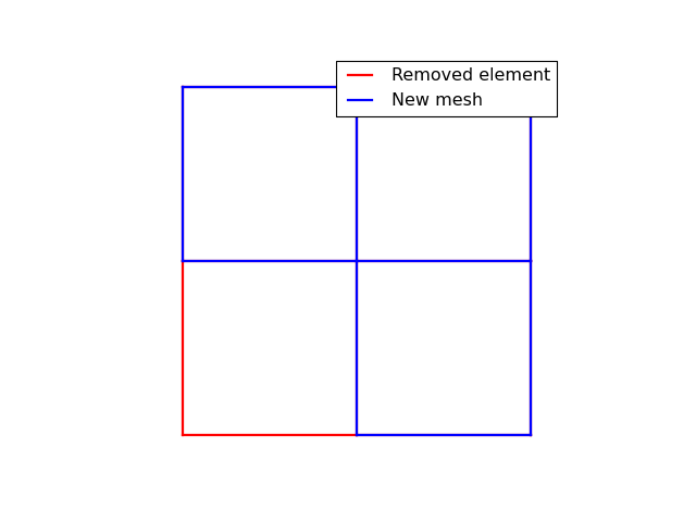
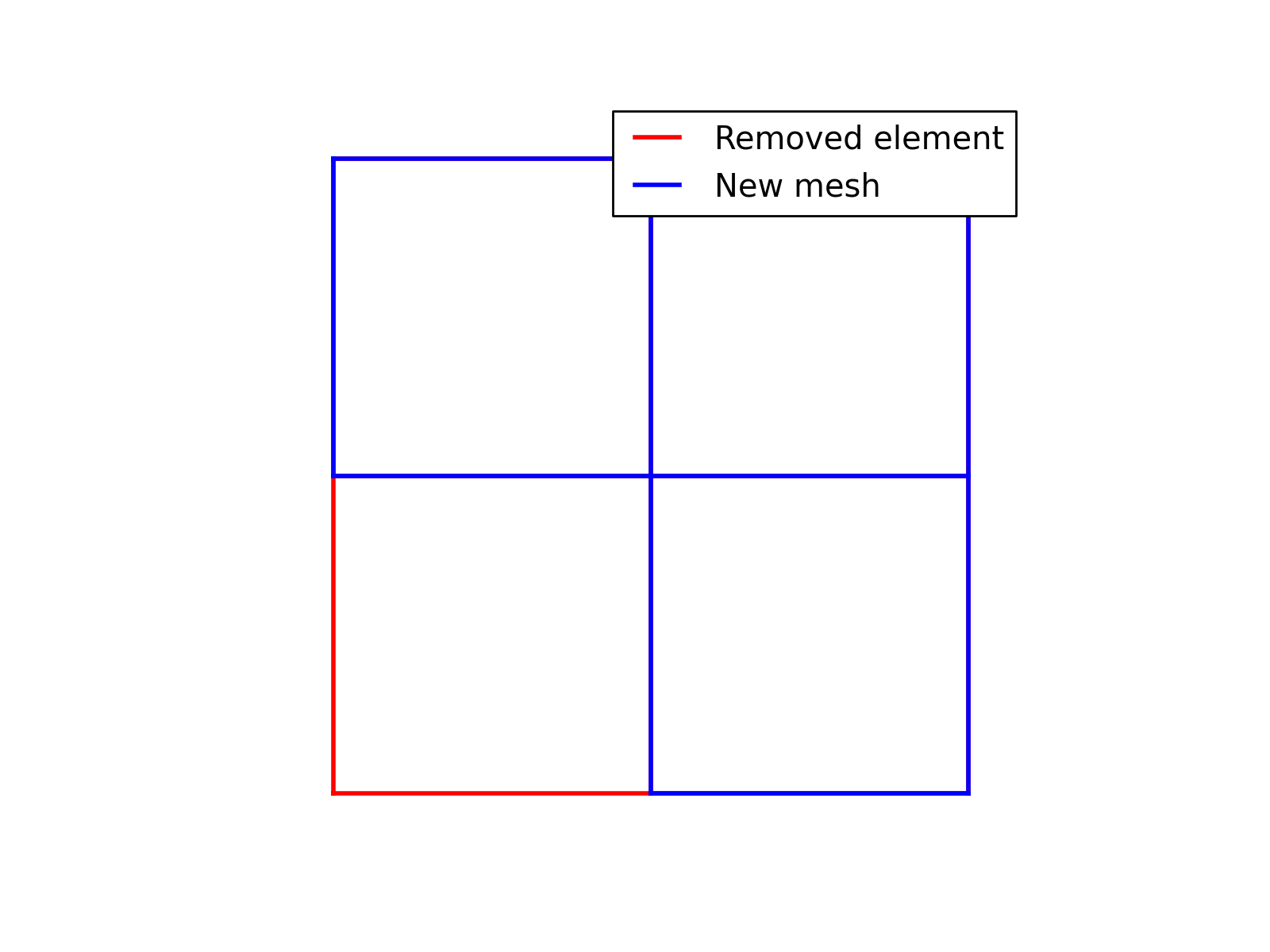
Mesh.drop_node(label)[source]¶ Drops a node from mesh.nodes instance. This method differs from to the nodes.drop_node element because it removes the node but also all elements containing the node in the mesh instance.
Parameters: label (int > 0) – node to be removed’s label. from abapy.mesh import RegularQuadMesh from matplotlib import pyplot as plt # Creating a mesh m = RegularQuadMesh(N1 = 2, N2 = 2) x0, y0, z0 = m.get_edges() # Finding the node located at x = y =0.: nodes = m.nodes for i in xrange(len(nodes.labels)): if nodes.x[i] == 0. and nodes.y[i] == 0.: node = nodes.labels[i] # Removing this node m.drop_node(node) x1, y1, z1 = m.get_edges() bbx, bby, bbz = m.nodes.boundingBox() plt.figure() plt.clf() plt.gca().set_aspect('equal') plt.axis('off') plt.xlim(bbx) plt.ylim(bby) plt.plot(x0,y0, 'r-', linewidth = 2., label = 'Removed element') plt.plot(x1,y1, 'b-', linewidth = 2., label = 'New mesh') plt.legend() plt.show()
(Source code, png, hires.png, pdf)

-
Mesh.add_set(label, elements)[source]¶ Adds a new set or appends elements to an existing set.
Parameters: - label (string) – set label to be added.
- elements (int > 0 or list of int > 0) – element(s) that belong to the step.
>>> from abapy.mesh import Mesh, Nodes
>>> mesh = Mesh()
>>> nodes = mesh.nodes
>>> # Adding some nodes
>>> nodes.add_node(label = 1, x = 0. ,y = 0. , z = 0.)
>>> nodes.add_node(label = 2, x = 1. ,y = 0. , z = 0.)
>>> nodes.add_node(label = 3, x = 1. ,y = 1. , z = 0.)
>>> nodes.add_node(label = 4, x = 0. ,y = 1. , z = 0.)
>>> nodes.add_node(label = 5, x = 2. ,y = 0. , z = 0.)
>>> nodes.add_node(label = 6, x = 2. ,y = 1. , z = 0.)
>>> # Adding some elements
>>> mesh.add_element(label=1, connectivity = (1,2,3,4), space =2, name = 'QUAD4')
>>> mesh.add_element(label=2, connectivity = (2,5,6,3), space =2, name = 'QUAD4')
>>> # Adding sets
>>> mesh.add_set(label = 'niceSet', elements = 1)
>>> mesh.add_set(label = 'veryNiceSet', elements = [1,2])
>>> mesh.add_set(label = 'simplyTheBestSet', elements = 1)
>>> mesh.add_set(label = 'simplyTheBestSet', elements = 2)
>>> print mesh
Mesh class instance:
Elements:
Label       Connectivity            Space   Name
1   [1L, 2L, 3L, 4L]        2D      QUAD4
2   [2L, 5L, 6L, 3L]        2D      QUAD4
Sets:
Label       Elements
niceset     1
veryniceset 1,2
simplythebestset    1,2
-
Mesh.drop_set(label)[source]¶ Goal: drops a set without removing elements and nodes. Inputs:
- label: set label to be dropped, must be string.
-
Mesh.add_surface(label, description)[source]¶ Adds or expands an element surface (i. e. a group a element faces). Surfaces are used to define contact interactions in simulations.
Parameters: - label (string) – surface label.
- description (list containing tuples each containing a string and an int) – list of ( element set label , face number ) tuples.
>>> from abapy.mesh import RegularQuadMesh
>>> mesh = RegularQuadMesh()
>>> mesh.add_surface('topsurface', [ ('top', 1) ])
>>> mesh.add_surface('topsurface', [ ('top', 2) ])
>>> mesh.surfaces
{'topsurface': [('top', 1), ('top', 2)]}
-
Mesh.node_set_to_surface(surface, nodeSet)[source]¶ Builds a surface from a node set.
Parameters: - surface (string) – surface label
- nodeSet (string) – nodeSet label
from abapy import mesh

m = mesh.RegularQuadMesh(N1 = 4, N2 = 4, l1 = 2., l2 = 6.)
m.nodes.sets = {}
m.nodes.add_set_by_func("top_nodes", lambda x,y,z,labels : y == 6.)
m.node_set_to_surface("top_surface", "top_nodes")
-
Mesh.replace_node(old, new)[source]¶ Replaces a node of given label (old) by another existing node (new). This version of
replace_nodediffers from the version of theNodesclass because it also updates elements connectivity. When working with mesh (an not only nodes), this version should be used.Parameters: - old (int > 0) – node label to be replaced.
- new (int > 0) – node label of the node replacing old.
>>> from abapy.mesh import RegularQuadMesh
>>> N1, N2 = 1,1
>>> mesh = RegularQuadMesh(N1, N2)
>>> mesh.replace_node(1,2)
Info: element 1 maybe have become degenerate due du node replacing.
>>> print mesh
Mesh class instance:
Elements:
Label       Connectivity            Space   Name
1   [2L, 4L, 3L]    2D      QUAD4
Sets:
Label       Elements
Useful data
-
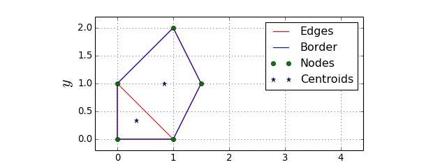
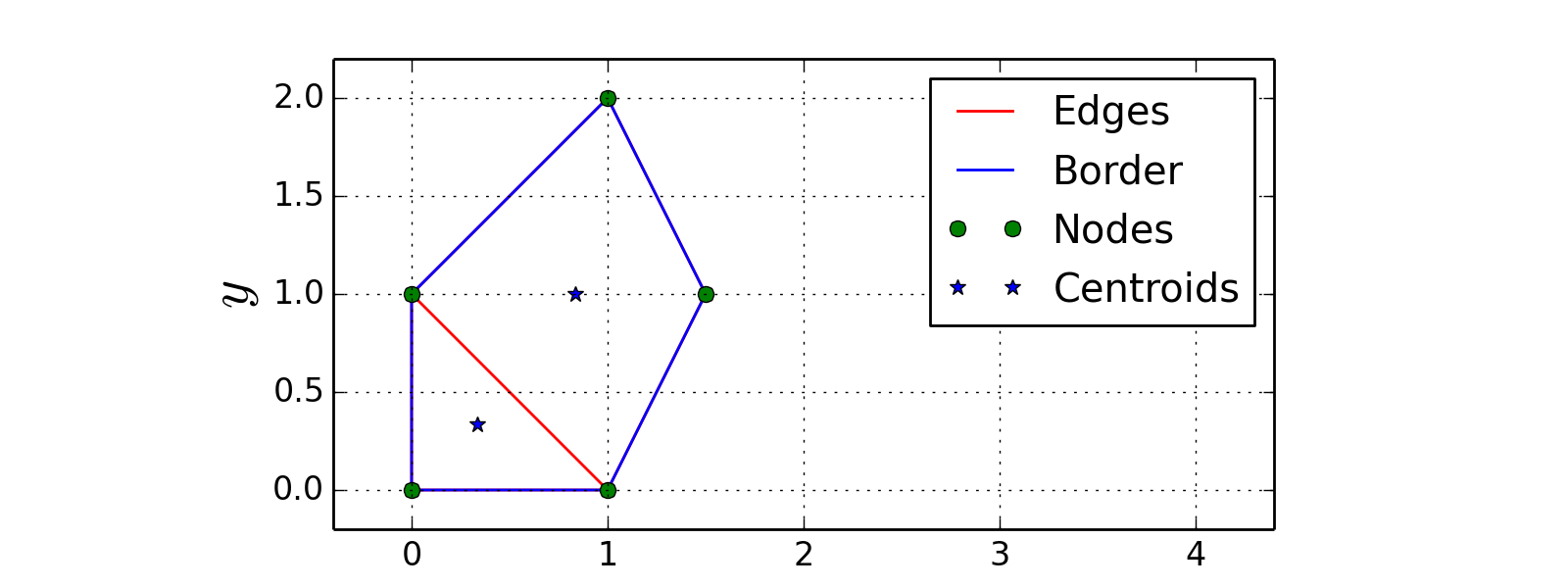
Mesh.centroids()[source]¶ Returns a dictionnary containing the coordinates of all the nodes belonging to earch element.
from abapy.mesh import Mesh
from matplotlib import pyplot as plt
import numpy as np

N1,N2 = 10,5 # Number of elements
l1, l2 = 4., 2. # Mesh size
fs = 20. # fontsize
mesh = Mesh()
nodes =  mesh.nodes
nodes.add_node(label = 1, x = 0., y = 0.)
nodes.add_node(label = 2, x = 1., y = 0.)
nodes.add_node(label = 3, x = 0., y = 1.)
nodes.add_node(label = 4, x = 1.5, y = 1.)
nodes.add_node(label = 5, x = 1., y = 2.)
mesh.add_element(label = 1, connectivity = [1,2,3], space = 2)
mesh.add_element(label = 2, connectivity = [2,4,5,3], space = 2)


centroids = mesh.centroids()

plt.figure(figsize=(8,3))
plt.gca().set_aspect('equal')
nodes = mesh.nodes
xn, yn, zn = np.array(nodes.x), np.array(nodes.y), np.array(nodes.z) # Nodes coordinates
xe,ye,ze = mesh.get_edges() # Mesh edges
xb,yb,zb = mesh.get_border() # Mesh border


plt.plot(xe,ye,'r-',label = 'Edges')
plt.plot(xb,yb,'b-',label = 'Border')
plt.plot(xn,yn,'go',label = 'Nodes')
plt.xlim([-.1*l1,1.1*l1])
plt.ylim([-.1*l2,1.1*l2])
plt.xlabel('$x$',fontsize = fs)
plt.ylabel('$y$',fontsize = fs)
plt.plot(centroids[:,0], centroids[:,1], '*', label = "Centroids")
plt.legend()
plt.grid()
plt.show()
(Source code, png, hires.png, pdf)

-
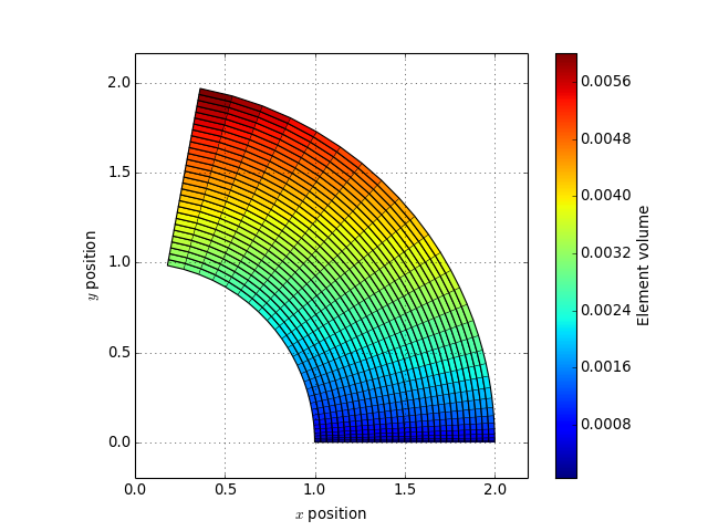
Mesh.volume()[source]¶ Returns a dictionnary containing the volume of all the elements.
from abapy.mesh import RegularQuadMesh
from abapy.indentation import IndentationMesh
import matplotlib.pyplot as plt
from matplotlib.path import Path
import matplotlib.patches as patches
import matplotlib.collections as collections
import numpy as np
from matplotlib import cm
from scipy import interpolate


def function(x, y, z, labels):
  r0 = 1.
  theta = .5 * np.pi * x
  r = y + r0
  ux = -x + r * np.cos(theta**2)
  uy = -y + r * np.sin(theta**2)
  uz = 0. * z
  return ux, uy, uz
N1, N2 = 30, 30
l1, l2 = .75, 1.


m = RegularQuadMesh(N1 = N1, N2 = N2, l1 = l1, l2 = l2)
vectorField = m.nodes.eval_vectorFunction(function)
m.nodes.apply_displacement(vectorField)
patches = m.dump2polygons()
volume = m.volume()
bb = m.nodes.boundingBox()
patches.set_facecolor(None) # Required to allow face color
patches.set_array(volume)
patches.set_linewidth(1.)
fig = plt.figure(0)
plt.clf()
ax = fig.add_subplot(111)
ax.set_aspect("equal")
ax.add_collection(patches)
plt.legend()
cbar = plt.colorbar(patches)
plt.grid()
plt.xlim(bb[0])
plt.ylim(bb[1])
plt.xlabel("$x$ position")
plt.ylabel("$y$ position")
cbar.set_label("Element volume")
plt.show()
(Source code, png, hires.png, pdf)
Modifications
-
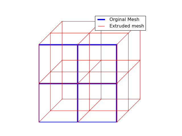
Mesh.extrude(N=1, l=1.0, quad=False, mapping={})[source]¶ Extrudes a mesh in z direction. The method is made to be applied to 2D mesh, it may work on shell elements but may lead to inside out elements.
Parameters: - N (int) – number of ELEMENTS along z, must > 0.
- l (float) – length of the extrusion along z, should be > 0 to avoid inside out elements.
- quad (boolean) – specifies if quadratic elements should be used instead of linear elements (default). Doesn’t work yet. Linear and quadratic elements should not be mixed in the same mesh.
- mapping (boolean) – gives the way to translate element names during extrusion. Example: {‘CAX4’:’C3D8’,’CAX3’:’C3D6’}. If 2D element name is not in the mapping, names will be chosen in the basic continuum elements used by Abaqus: ‘C3D6’ and ‘C3D8’.
from abapy.mesh import RegularQuadMesh, Mesh
from matplotlib import pyplot as plt

m = RegularQuadMesh(N1 = 2, N2 =2)
m.add_set('el_set',[1,2])
m.add_surface('my_surface',[('el_set',2), ])
m2 = m.extrude(l = 1., N = 2)
x,y,z = m.get_edges()
x2,y2,z2 = m2.get_edges()

# Adding some 3D "home made" perspective:
zx, zy = .3, .3
for i in xrange(len(x2)):
  if x2[i] != None:
    x2[i] += zx * z2[i]
    y2[i] += zy * z2[i]

# Plotting stuff
plt.figure()
plt.clf()
plt.gca().set_aspect('equal')
plt.axis('off')
plt.plot(x,y, 'b-', linewidth  = 4., label = 'Orginal Mesh')
plt.plot(x2,y2, 'r-', linewidth  = 1., label = 'Extruded mesh')
plt.legend()
plt.show()
(Source code, png, hires.png, pdf)

-
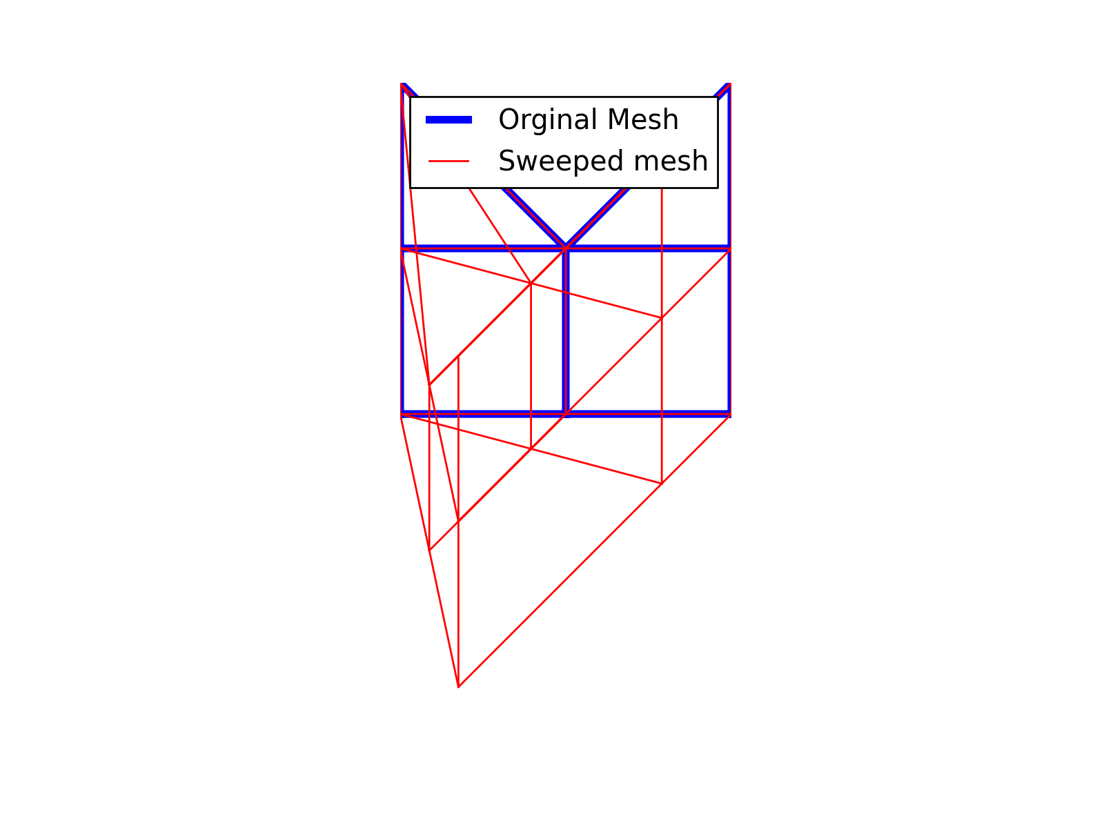
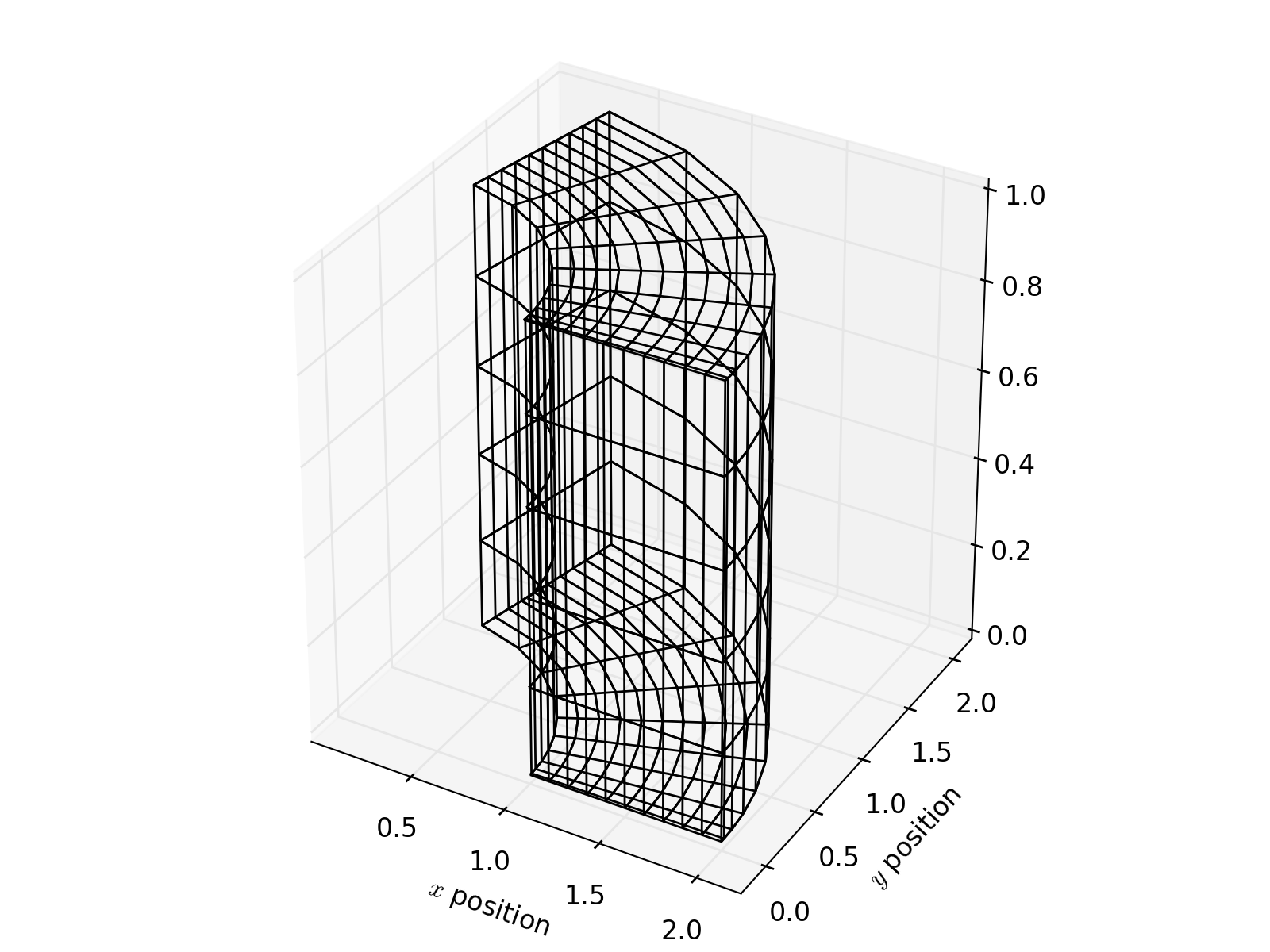
Mesh.sweep(N=1, sweep_angle=45.0, quad=False, mapping={}, extrude=False)[source]¶ Sweeps a mesh in around z axis. The method is made to be applied to 2D mesh, it may work on shell elements but may lead to inside out elements.
Parameters: - N (int) – number of ELEMENTS along z, must > 0.
- sweep_angle (float) – sweep angle around the z axis in degrees. Should be > 0 to avoid inside out elements.
- quad (boolean) – specifies if quadratic elements should be used instead of linear elements (default). Doesn’t work yet. Linear and quadratic elements should not be mixed in the same mesh.
- mapping (dictionary) – gives the way to translate element names during extrusion. Example: {‘CAX4’:’C3D8’,’CAX3’:’C3D6’}. If 2D element name is not in the mapping, names will be chosen in the basic continuum elements used by Abaqus: ‘C3D6’ and ‘C3D8’.
- extrude (boolean) – if True, this param will modify the transformation used to produce the sweep. The result will be a mixed form of sweep and extrusion useful to produce pyramids. When using this option, the sweep angle must be lower than 90 degrees.
from abapy.mesh import RegularQuadMesh, Mesh
from matplotlib import pyplot as plt
from array import array
from abapy.indentation import IndentationMesh

m = RegularQuadMesh(N1 = 2, N2 =2)
m.connectivity[2] = array(m.dti,[5, 7, 4])
m.connectivity[3] = array(m.dti,[5, 6, 9])
m.add_set('el_set',[1,2])
m.add_set('el_set2',[2,4])
m.add_surface('my_surface',[('el_set',1),])
m2 = m.sweep(sweep_angle = 70., N = 2, extrude=True)
x,y,z = m.get_edges()
x2,y2,z2 = m2.get_edges()

# Adding some 3D "home made" perspective:
zx, zy = .3, .3
for i in xrange(len(x2)):
  if x2[i] != None:
    x2[i] += zx * z2[i]
    y2[i] += zy * z2[i]

# Plotting stuff
plt.figure()
plt.clf()
plt.gca().set_aspect('equal')
plt.axis('off')
plt.plot(x,y, 'b-', linewidth  = 4., label = 'Orginal Mesh')
plt.plot(x2,y2, 'r-', linewidth  = 1., label = 'Sweeped mesh')
plt.legend()
plt.show()
(Source code, png, hires.png, pdf)

-
Mesh.union(other_mesh, crit_distance=None, simplify=True)[source]¶ Computes the union of 2 Mesh instances. The second operand’s labels are increased to be compatible with the first. All sets are kepts and merged if they share the same name. Nodes which are too close (< crit_distance) are merged. If crit_distance is None, the defautl value value of
simplify_meshis used.Parameters: - other_mesh (
Meshinstance) – mesh to be added to current mesh. - crit_distance (float > 0) – critical distance under which nodes are considered identical.
- other_mesh (
-
Mesh.apply_reflection(point=(0.0, 0.0, 0.0), normal=(1.0, 0.0, 0.0))[source] Applies a reflection symmetry to the mesh instance. The reflection plane is defined by a point and a normal direction.
Parameters: - point (tuple or list containing 3 floats) – coordinates of a point of the reflection plane.
- normal (tuple or list containing 3 floats) – normal vector to the reflection plane
Return type: Meshinstance..note: This method can lead to coherence problems with surfaces, this problem will be addressed in the future. Surfaces are removed by this operation untill this problem is solved.
from abapy.mesh import RegularQuadMesh
from abapy.indentation import ParamInfiniteMesh
import matplotlib.pyplot as plt

point  = (0., 0., 0.)
normal = (1., 0., 0.)
m0 = ParamInfiniteMesh()
x0, y0, z0 = m0.get_edges()
m1 = m0.apply_reflection(normal = normal, point = point)
x1, y1, z1 = m1.get_edges()
plt.plot(x0, y0)
plt.plot(x1, y1)
plt.gca().set_aspect('equal')
plt.show()
(Source code, png, hires.png, pdf)
Export
-
Mesh.dump2inp()[source]¶ Dumps the whole mesh (i. e. elements + nodes) to Abaqus INP format.
Return type: string >>> from abapy.mesh import Mesh, Nodes >>> mesh = Mesh() >>> nodes = mesh.nodes >>> # Adding some nodes >>> nodes.add_node(label = 1, x = 0. ,y = 0. , z = 0.) >>> nodes.add_node(label = 2, x = 1. ,y = 0. , z = 0.) >>> nodes.add_node(label = 3, x = 1. ,y = 1. , z = 0.) >>> nodes.add_node(label = 4, x = 0. ,y = 1. , z = 0.) >>> nodes.add_node(label = 5, x = 2. ,y = 0. , z = 0.) >>> nodes.add_node(label = 6, x = 2. ,y = 1. , z = 0.) >>> # Adding some elements >>> mesh.add_element(label=1, connectivity = (1,2,3,4), space =2, name = 'QUAD4') >>> mesh.add_element(label=2, connectivity = (2,5,6,3), space =2, name = 'QUAD4') >>> # Adding sets >>> mesh.add_set(label = 'veryNiceSet', elements = [1,2]) >>> # Adding surfaces >>> mesh.add_surface(label = 'superNiceSurface', description = [ ('veryNiceSet', 2) ]) >>> out = mesh.dump2inp()
-
Mesh.dump2vtk(path=None)[source]¶ Dumps the mesh to the VTK format. VTK format can be visualized using Mayavi2 or Paraview. This method is particularly useful for 3D mesh. For 2D mesh, it may be more efficient to work with matplotlib using methods like: get_edges, get_border and dump2triplot.
Parameters: path – if None, return a string containing the VTK data. If not, must be a path to a file where the data will be written. Return type: string or None. from abapy.mesh import RegularQuadMesh from abapy.indentation import IndentationMesh import numpy as np def tensor_function(x, y, z, labels): """ Vector function used to produced the displacement field. """ r0 = 1. theta = .5 * np.pi * x r = y + r0 s11 = z + x s22 = z + y s33 = x**2 s12 = y**2 s13 = x + y s23 = z return s11, s22, s33, s12, s13, s23 def vector_function(x, y, z, labels): """ Vector function used to produced the displacement field. """ r0 = 1. theta = .5 * np.pi * x r = y + r0 ux = -x + r * np.cos(theta**2) uy = -y + r * np.sin(theta**2) uz = 0. * z return ux, uy, uz def scalar_function(x, y, z, labels): """ Scalar function used to produced the plotted field. """ return x**2 + y**2 #MESH GENERATION N1, N2, N3 = 8, 8, 8 l1, l2, l3 = .75, 1., .5 m = RegularQuadMesh(N1 = N1, N2 = N2, l1 = l1, l2 = l2).extrude(N = N3, l = l3) #FIELDS GENERATION s = m.nodes.eval_tensorFunction(tensor_function) m.add_field(s, "s") u = m.nodes.eval_vectorFunction(vector_function) m.add_field(u, "u") m.nodes.apply_displacement(u) f = m.nodes.eval_function(scalar_function) m.add_field(f, "f") m.dump2vtk("Mesh-dump2vtk.vtk")
- VTK output:
Mesh-dump2vtk.vtk - Paraview plot:
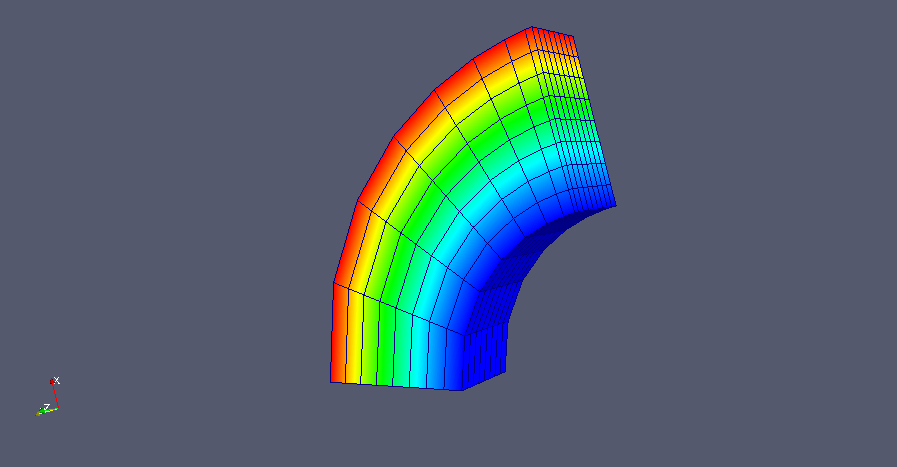
- VTK output:
Ploting tools
-
Mesh.convert2tri3(mapping=None)[source]¶ Converts 2D elements to 3 noded triangles only.
Parameters: mapping (dict with string keys and values) – gives the mapping of element name changes to be applied when elements are splitted. Example: mapping = {‘CAX4’:’CAX3’} Return type: Mesh instance containing only triangular elements. Note
This function was mainly developped to allow easy ploting in matplotlib using
matplotlib.plyplot.triplot,matplotlib.plyplot.tricontourandmatplotlib.plyplot.contourfwhich rely on full triangle meshes. On a practical point of view, it easily used wrapped inside theabapy.Mesh.dump2triplotmethods which rewrites connectivity in an easier to plot way.from abapy.mesh import Mesh, Nodes, RegularQuadMesh import matplotlib.pyplot as plt from numpy import cos, pi def function(x, y, z, labels): r = (x**2 + y**2)**.5 return cos(2*pi*x)*cos(2*pi*y)/(r+1.) N1, N2 = 30, 30 l1, l2 = 1., 1. Ncolor = 10 mesh = RegularQuadMesh(N1 = N1, N2 = N2, l1 = l1, l2 = l2) field = mesh.nodes.eval_function(function) fig = plt.figure(figsize=(16,4)) ax = fig.add_subplot(131) ax2 = fig.add_subplot(132) ax3 = fig.add_subplot(133) ax.set_aspect('equal') ax2.set_aspect('equal') ax3.set_aspect('equal') ax.set_xticks([]) ax.set_yticks([]) ax2.set_xticks([]) ax2.set_yticks([]) ax3.set_xticks([]) ax3.set_yticks([]) ax.set_frame_on(False) ax2.set_frame_on(False) ax3.set_frame_on(False) ax.set_title('Orginal Mesh') ax2.set_title('Triangularized Mesh') ax3.set_title('Field') x,y,z = mesh.get_edges() # Mesh edges xt,yt,zt = mesh.convert2tri3().get_edges() # Triangular mesh edges xb,yb,zb = mesh.get_border() X,Y,Z,tri = mesh.dump2triplot() ax.plot(x,y,'k-') ax2.plot(xt,yt,'k-') ax3.plot(xb,yb,'k-', linewidth = 2.) ax3.tricontourf(X,Y,tri,field.data, Ncolor) ax3.tricontour(X,Y,tri,field.data, Ncolor, colors = 'black') ax.set_xlim([-.1*l1,1.1*l1]) ax.set_ylim([-.1*l2,1.1*l2]) ax2.set_xlim([-.1*l1,1.1*l1]) ax2.set_ylim([-.1*l2,1.1*l2]) ax3.set_xlim([-.1*l1,1.1*l1]) ax3.set_ylim([-.1*l2,1.1*l2]) plt.show()
-
Mesh.dump2triplot(use_3D=False)[source]¶ Allows any 2D mesh to be triangulized and formated in a suitable way to be used by triplot, tricontour and tricontourf in matplotlib.pyplot. This is the best way to produce clean 2D plots of 2D meshs. Returns 4 arrays/lists: x, y and z coordinates of nodes and triangles connectivity. It can be directly used in matplotlib.pyplot using:
Return type: 4 lists >>> import matplotlib.pyplot as plt >>> from abapy.mesh import RegularQuadMesh >>> plt.figure() >>> plt.axis('off') >>> plt.gca().set_aspect('equal') >>> mesh = RegularQuadMesh(N1 = 10 , N2 = 10) >>> x,y,z,tri = mesh.dump2triplot() >>> plt.triplot(x,y,tri) >>> plt.show()
-
Mesh.get_edges(xmin=None, xmax=None, ymin=None, ymax=None, zmin=None, zmax=None)[source]¶ Returns the list of edges composing the meshed domain. Edges are given as x and y lists with None separator for faster ploting in
matplotlib.pyplot.Return type: 3 lists of coordinates directly plotable in matplotlib
-
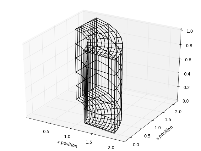
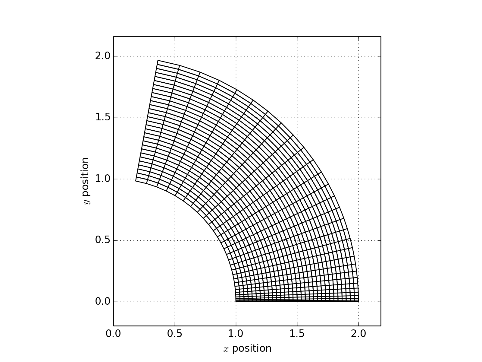
Mesh.dump2polygons(edge_color='black', edge_width=1.0, face_color=None, use_3D=False)[source]¶ Returns 2D elements as matplotlib poly collection.
Parameters: - edge_color – edge color.
- edge_width – edge width.
- face_color – face color.
- use_3D – True for 3D polygon export.
from abapy.mesh import RegularQuadMesh
from abapy.indentation import IndentationMesh
import matplotlib.pyplot as plt
from matplotlib.path import Path
import matplotlib.patches as patches
import matplotlib.collections as collections
import numpy as np
from matplotlib import cm
from scipy import interpolate


def function(x, y, z, labels):
  r0 = 1.
  theta = .5 * np.pi * x
  r = y + r0
  ux = -x + r * np.cos(theta**2)
  uy = -y + r * np.sin(theta**2)
  uz = 0. * z
  return ux, uy, uz
N1, N2 = 30, 30
l1, l2 = .75, 1.


m = RegularQuadMesh(N1 = N1, N2 = N2, l1 = l1, l2 = l2)
vectorField = m.nodes.eval_vectorFunction(function)
m.nodes.apply_displacement(vectorField)
patches = m.dump2polygons()
bb = m.nodes.boundingBox()
patches.set_linewidth(1.)
fig = plt.figure(0)
plt.clf()
ax = fig.add_subplot(111)
ax.set_aspect("equal")
ax.add_collection(patches)
plt.grid()
plt.xlim(bb[0])
plt.ylim(bb[1])
plt.xlabel("$x$ position")
plt.ylabel("$y$ position")
plt.show()
(Source code, png, hires.png, pdf)

from abapy.mesh import RegularQuadMesh
from abapy.indentation import IndentationMesh
import matplotlib.pyplot as plt
from matplotlib.path import Path
import matplotlib.patches as patches
import matplotlib.collections as collections
import mpl_toolkits.mplot3d as a3
import numpy as np
from matplotlib import cm
from scipy import interpolate


def function(x, y, z, labels):
  r0 = 1.
  theta = .5 * np.pi * x
  r = y + r0
  ux = -x + r * np.cos(theta**2)
  uy = -y + r * np.sin(theta**2)
  uz = 0. * z
  return ux, uy, uz
N1, N2, N3 = 10, 10, 5
l1, l2, l3 = .75, 1., 1.


m = RegularQuadMesh(N1 = N1, N2 = N2, l1 = l1, l2 = l2)
m = m.extrude(l = l3, N = N3 )
vectorField = m.nodes.eval_vectorFunction(function)
m.nodes.apply_displacement(vectorField)
patches = m.dump2polygons(use_3D = True,
                          face_color = None,
                          edge_color = "black")
bb = m.nodes.boundingBox()
patches.set_linewidth(1.)

fig = plt.figure(0)
plt.clf()
ax = a3.Axes3D(fig)
ax.set_aspect("equal")
ax.add_collection3d(patches)
plt.xlim(bb[0])
plt.ylim(bb[1])
plt.xlabel("$x$ position")
plt.ylabel("$y$ position")
plt.show()
(Source code, png, hires.png, pdf)
-
Mesh.draw(ax, field_func=None, disp_func=None, cmap=None, cmap_levels=20, cbar_label='Field', cbar_orientation='horizontal', edge_color='black', edge_width=1.0, node_style='k.', node_size=1.0, contour=False, contour_colors='black', alpha=1.0)[source]¶ Draws a 2D mesh in a given matplotlib axes instance.
Parameters: - ax – matplotlib axes instance.
- field_func (function or None) – a function that defines how to used existing fields to produce a FieldOutput instance.
- disp_func (function) – a function that defines how to used existing fields to produce a VectorFieldOutput instance used as a diplacement field.
- cmap – matplotlib colormap.
- cmap_levels – number of levels in the colormap
- cbar_label (string) – colorbar label.
- cbar_orientation – “horizontal” or “vertical”.
- edge_color – valid matplotlib color for the edges of the mesh.
- edge_width – mesh edge width.
- node_style – nodes plot style.
- node_size – nodes size.
- contour (boolean) – plot field contour.
- contour_colors – contour colors to use, colormap of fixed color.
- alpha – alpha lvl of the gradiant plot.
from abapy.mesh import RegularQuadMesh
from abapy.indentation import IndentationMesh
import matplotlib.pyplot as plt
from matplotlib.path import Path
import matplotlib.patches as patches
import matplotlib.collections as collections
import numpy as np
from matplotlib import cm
from scipy import interpolate

def vector_function(x, y, z, labels):
  """
  Vector function used to produced the displacement field.
  """
  r0 = 1.
  theta = .5 * np.pi * x
  r = y + r0
  ux = -x + r * np.cos(theta**2)
  uy = -y + r * np.sin(theta**2)
  uz = 0. * z
  return ux, uy, uz

def scalar_function(x, y, z, labels):
  """
  Scalar function used to produced the plotted field.
  """
  return x**2 + y**2
#MESH GENERATION
N1, N2 = 30, 30
l1, l2 = .75, 1.
m = RegularQuadMesh(N1 = N1, N2 = N2, l1 = l1, l2 = l2)
#FIELDS GENERATION
u = m.nodes.eval_vectorFunction(vector_function)
m.add_field(u, "u")
f = m.nodes.eval_function(scalar_function)
m.add_field(f, "f")
#PLOTS
fig = plt.figure(0)
plt.clf()
ax = fig.add_subplot(1,1,1)
m.draw(ax,
    disp_func  = lambda fields : fields["u"],
    field_func = lambda fields : fields["f"],
    cmap = cm.jet,
    cbar_orientation = "vertical",
    contour = False,
    contour_colors = "black",
    alpha = 1.,
    cmap_levels = 10,
    edge_width = .1)
ax.set_aspect("equal")
plt.grid()
plt.xlabel("$x$ position")
plt.ylabel("$y$ position")
plt.show()
Mesh generation
RegularQuadMesh functions
-
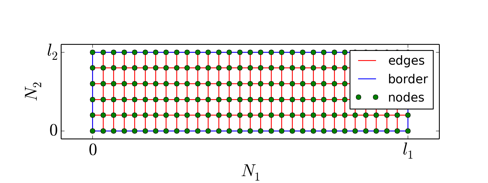
abapy.mesh.RegularQuadMesh(N1=1, N2=1, l1=1.0, l2=1.0, name='QUAD4', dtf='f', dti='I')[source]¶ Generates a 2D regular quadrangle mesh.
Parameters: - N1 (int > 0) – number of elements respectively along y.
- N2 (int > 0) – number of elements respectively along y.
- l1 (float) – length of the mesh respectively along x.
- l2 (float) – length of the mesh respectively along y.
- name (string) – elements names, for example ‘CPS4’.
- dti ('I', 'H') – int data type in array.array
- dtf ('f', 'd') – float data type in array.array
Return type: Mesh instance
from abapy.mesh import RegularQuadMesh
from matplotlib import pyplot as plt
N1,N2 = 30,5 # Number of elements
l1, l2 = 4., 1. # Mesh size
fs = 20. # fontsize
mesh = RegularQuadMesh(N1,N2,l1,l2)
plt.figure(figsize=(8,3))
plt.gca().set_aspect('equal')
nodes = mesh.nodes
xn, yn, zn = nodes.x, nodes.y, nodes.z # Nodes coordinates
xe,ye,ze = mesh.get_edges() # Mesh edges
xb,yb,zb = mesh.get_border() # Mesh border
plt.plot(xe,ye,'r-',label = 'edges')
plt.plot(xb,yb,'b-',label = 'border')
plt.plot(xn,yn,'go',label = 'nodes')
plt.xlim([-.1*l1,1.1*l1])
plt.ylim([-.1*l2,1.1*l2])
plt.xticks([0,l1],['$0$', '$l_1$'],fontsize = fs)
plt.yticks([0,l2],['$0$', '$l_2$'],fontsize = fs)
plt.xlabel('$N_1$',fontsize = fs)
plt.ylabel('$N_2$',fontsize = fs)
plt.legend()
plt.show()
(Source code, png, hires.png, pdf)
-
abapy.mesh.RegularQuadMesh_like(x_list=[0.0, 1.0], y_list=[0.0, 1.0], name='QUAD4', dtf='f', dti='I')[source]¶ Generates a 2D regular quadrangle mesh from 2 lists of positions. This version of RegularQuadMesh is an alternative to the normal one in some cases where fine tuning of x, y positions is required.
Parameters: - x_list (list, array.array or numpy.array) – list of x values
- y_list (list, array.array or numpy.array) – list of y values
- name (string) – elements names, for example ‘CPS4’.
- dti ('I', 'H') – int data type in array.array
- dtf ('f', 'd') – float data type in array.array
Return type: Mesh instance
Other meshes
-
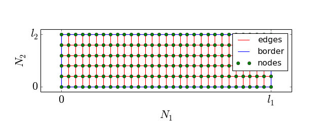
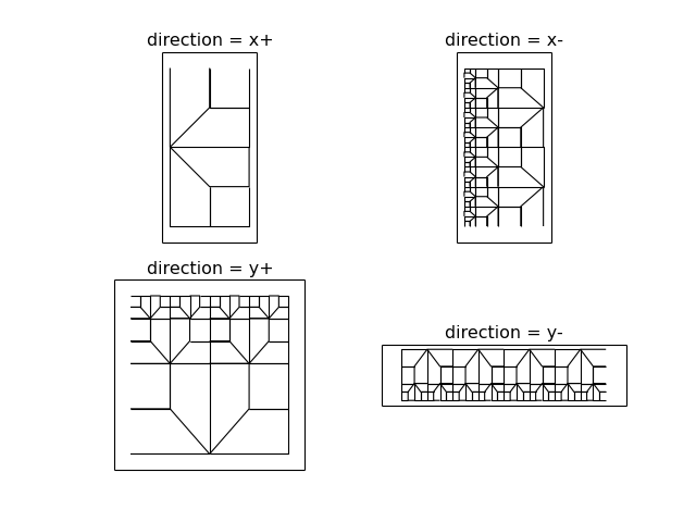
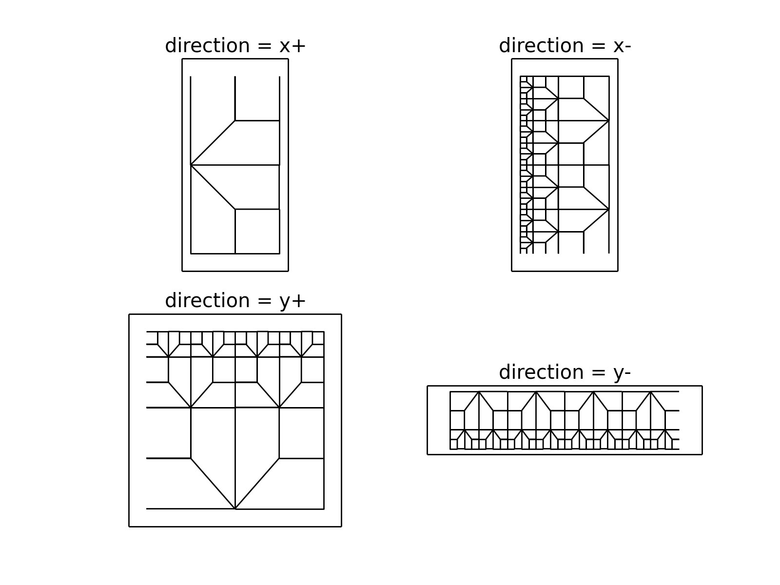
abapy.mesh.TransitionMesh(N1=4, N2=2, l1=1.0, l2=1.0, direction='y+', name='CAX4', crit_distance=1e-06)[source]¶ A mesh transition to manage them all...
Parameters: - N1 (int) – starting number of elements, must be multiple of 4.
- N2 (int) – ending number of elements, must be lower than N1 and multiple of 2.
- l1 (float) – length of the mesh in the x direction.
- l2 (float) – length of the mesh in the y direction.
- direction (str) – direction of mesh. Must be in (“x+”, “x-”, “y+”, “y-”).
- name (str) – name of the element in the export procedures.
- crit_distance (float) – critical distance in union process.
from abapy.mesh import TransitionMesh
from matplotlib import pyplot as plt

fig = plt.figure(0)
plt.clf()

ax = fig.add_subplot(221)
ax.set_aspect("equal")
ax.set_title('direction = x+')
m = TransitionMesh(N1 = 4, N2 = 2,l1 = 1., l2 = 2., direction = "x+")
patches = m.dump2polygons()
bb = m.nodes.boundingBox()
patches.set_linewidth(1.)
ax.add_collection(patches)
plt.xlim(bb[0])
plt.ylim(bb[1])
plt.xticks([])
plt.yticks([])

ax = fig.add_subplot(222)
ax.set_aspect("equal")
ax.set_title('direction = x-')
m = TransitionMesh(N1 =32, N2 = 4,l1 = 1., l2 = 2., direction = "x-")
patches = m.dump2polygons()
bb = m.nodes.boundingBox()
patches.set_linewidth(1.)
ax.add_collection(patches)
plt.xlim(bb[0])
plt.ylim(bb[1])
plt.xticks([])
plt.yticks([])

ax = fig.add_subplot(223)
ax.set_aspect("equal")
ax.set_title('direction = y+')
m = TransitionMesh(N1 = 16, N2 = 2,l1 = 1, l2 = 1., direction = "y+")
patches = m.dump2polygons()
bb = m.nodes.boundingBox()
patches.set_linewidth(1.)
ax.add_collection(patches)
plt.xlim(bb[0])
plt.ylim(bb[1])
plt.xticks([])
plt.yticks([])

ax = fig.add_subplot(224)
ax.set_aspect("equal")
ax.set_title('direction = y-')
m = TransitionMesh(N1 =32, N2 = 8,l1 = 4., l2 = 1., direction = "y-")
patches = m.dump2polygons()
bb = m.nodes.boundingBox()
patches.set_linewidth(1.)
ax.add_collection(patches)
plt.xlim(bb[0])
plt.ylim(bb[1])
plt.xticks([])
plt.yticks([])

plt.show()
(Source code, png, hires.png, pdf)

Note
see also in abapy.indentation for indentation dedicated meshes.