Indentation¶

Indentation simulation tools

Indentation meshes¶

`ParamInfiniteMesh` function¶

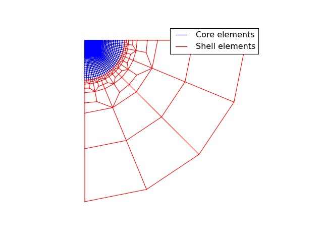
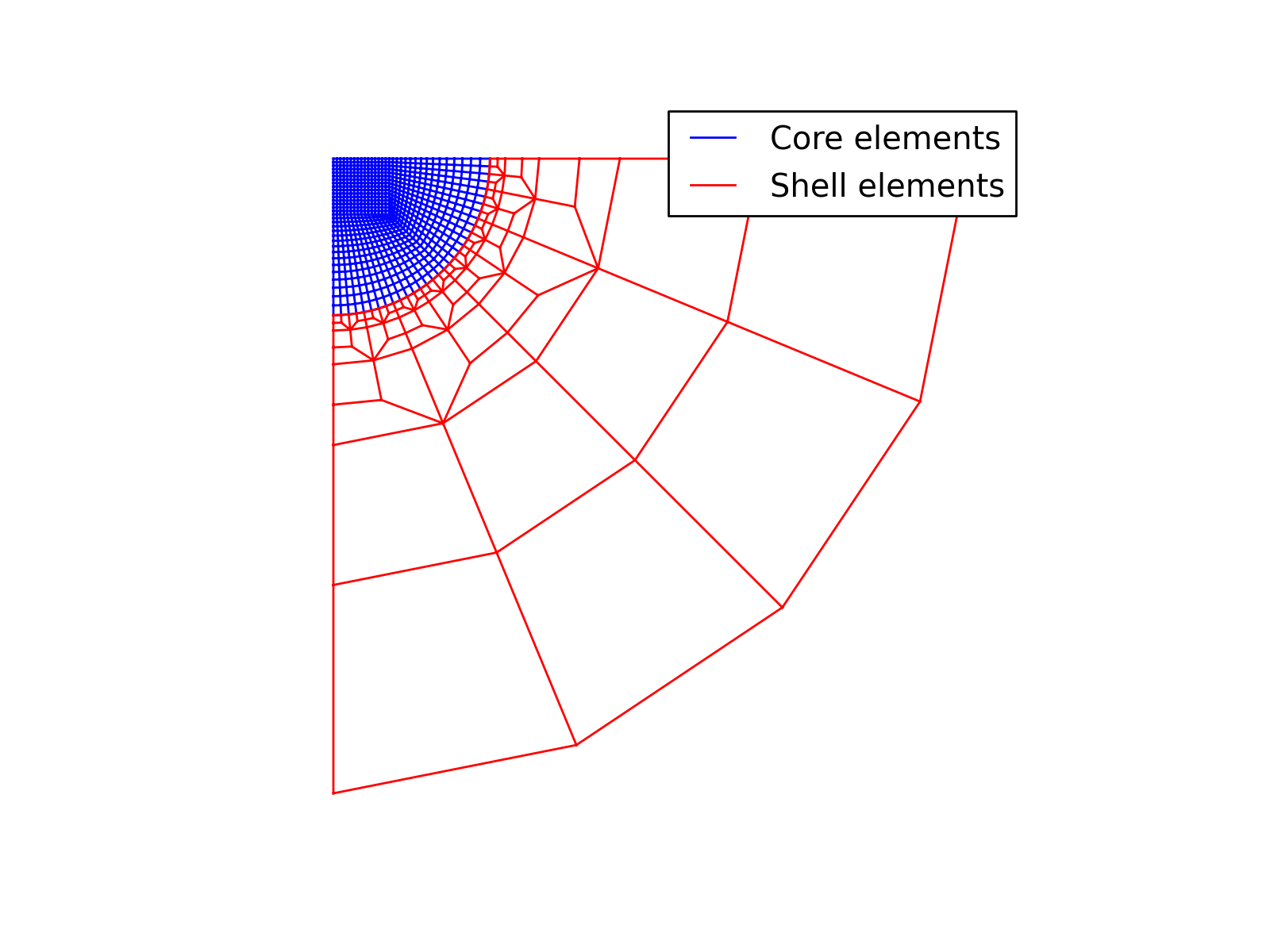
abapy.indentation.ParamInfiniteMesh(Na=10, Nb=10, l=1.0, core_name='CAX4', add_shell=True, shell_name='CINAX4', dti='I', dtf='d')[source]¶

Returns a mesh dedicated to 2D/Axisymmetrical indentation. It is composed of a core of quadrangle elements and a shell of infinite elements. The core is divided into three zones. The center is core_1, the right is core_2 and the bottom is core_3. Core_1 is a Na x Na square mesh whereas core_2 and core_3 are respectively Nb x Na and Na x Nb structured meshes that have been transformed to be connected and guaranty element size progression.

Parameters:	Na (int > 1) – number of elements per side in core_1 Nb (int > 0) – number of radial elements in core_2 and core_3 l (float > 0) – core_1 size core_name (string) – element name in core add_shell (boolean) – True if the shell of infinite elements is to be used, False if not. shell_name (string) – element name in shell, should be infinite

`IndentationMesh` function¶

abapy.indentation.IndentationMesh(Na=8, Nb=8, Ns=4, Nf=2, l=1.0, name='CAX4', dtf='f', dti='I')[source]¶

An indentation oriented full quad mesh.

Parameters:

Na (int) – number of elements along x axis in the finely meshed contact zone. Must be power of 2.
Nb (int) – number of elements along y axis in the finely meshed contact zone. Must be power of 2.
Ns (int) – number of radial elements in the shell.
Nf (int) – number of orthoradial elements in each half shell. Must be > 0.
l (float.) – length of the square zone.
name (string) – name of the elements. Note that this mesh if full quad so only one name is required.
dtf (string) – float data type in array.array, ‘d’ for float64 or ‘f’ for float32.
dti (string) – int data type in array.array, ‘I’ for unsignedint32 or ‘H’ for unsignedint16 (dangerous in some cases).

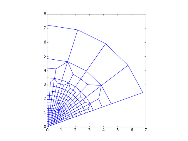
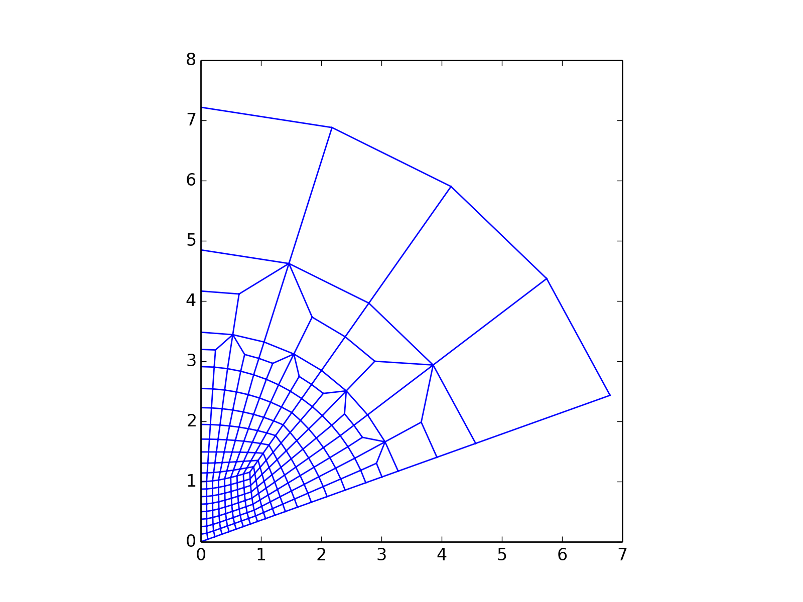
from abapy.indentation import IndentationMesh
from matplotlib import pyplot as plt

Na = 16 # Elements along x axis in the square zone
Nb = 16 # Elements along y axis in the square zone
Ns = 2 # Radial number of elements in the shell
Nf = 2 # Minimal number of orthoradial elements in heach half shell
l = 1. # Size of the square zone
name = 'CAX4' # Name of the elements

m = IndentationMesh(Na = Na, Nb = Nb, Ns = Ns, Nf= Nf, l = l, name = name)

m_core = m['core_elements']
m_shell = m['shell_elements']

x_core, y_core, z_core = m_core.get_edges()
x_shell, y_shell, z_shell = m_shell.get_edges()
plt.figure(0)
plt.clf()
plt.axis('off')
plt.grid()
xlim, ylim, zlim = m.nodes.boundingBox()
plt.gca().set_aspect('equal')
plt.xlim(xlim)
plt.ylim(ylim)
plt.plot(x_core,y_core, 'b-', label = 'Core elements')
plt.plot(x_shell,y_shell, 'r-', label = 'Shell elements')
plt.legend()
plt.show()

(Source code, png, hires.png, pdf)

Indenters¶

`RigidCone2D` class¶

class abapy.indentation.RigidCone2D(half_angle=70.3, width=10.0, summit_position=(0.0, 0.0))[source]¶

A rigid cone usable in 2D and Axisymmetric simulations.

Parameters:	half_angle (float > 0.) – half_angle in DEGREES. width (float > 0.) – width of the indenter summit_position (tuple or list containing two floats.) – position of the summit in a 2D space.

apply_displacement(disp)[source]¶

Applies a displacement field to the indenter.

Parameters:	disp (`abapy.postproc.VectorFieldOutput` instance.) – displacement field (with only one location).

dump2inp()[source]¶

Dumps to Abaqus INP format.

Return type:	string

get_edges()[source]¶

Returns a plotable version of the indenter usable directly in matplotlib.pyplot.

Return type:	x and y lists

set_half_angle(half_angle=70.3)[source]¶

Sets the half angle of the indenter. Default is equivalent to modified Berkovich indenter in volume.

Parameters:	half_angle (float > 0.) – half_angle in DEGREES.

set_summit_position(summit_position)[source]¶

Sets the position of the indenter.

Parameters:	summit_position (tuple or list containing two floats.) – position of the summit in a 2D space.

set_width(width)[source]¶

Sets the width of the indenter.

Parameters:	width (float > 0.) – width

`DeformableCone2D` class¶

class abapy.indentation.DeformableCone2D(half_angle=70.3, Na=4, Nb=4, Ns=4, Nf=2, l=1.0, mat_label='INDENTER_MAT', summit_position=(0.0, 0.0), rigid=False)[source]¶

A deformable cone usable in 2D and Axisymmetric simulations.

Parameters:

half_angle (float > 0.) – half_angle in DEGREES.
Na (int) – number of elements along x axis in the finely meshed contact zone. Must be power of 2.
Nb (int) – number of elements along y axis in the finely meshed contact zone. Must be power of 2.
Ns (int) – number of radial elements in the shell.
Nf (int) – number of orthoradial elements in each half shell. Must be > 0.
l (float.) – length of the square zone.
mat_label (any material class instance) – label of the constitutive material of the indenter.
summit_position (tuple or list containing two floats.) – position of the summit in a 2D space.
rigid – True if indenter is to be rigid or False if the indenter is to be deformable. If the rigid behavior is chosen, the material label will be necessary but will not influence the results of the simulation.

from abapy.indentation import DeformableCone2D
from matplotlib import pyplot as plt
c = DeformableCone2D(Na =8, Nb = 8, Ns = 1)
f = open('DeformableCone2D.inp', 'w')
f.write(c.dump2inp())
f.close()
x,y,z = c.mesh.get_edges()
plt.plot(x,y)
plt.gca().set_aspect('equal')
plt.show()

(Source code, png, hires.png, pdf)

apply_displacement(disp)[source]¶

Applies a displacement field to the indenter.

Parameters:	disp (`abapy.postproc.VectorFieldOutput` instance.) – displacement field (with only one location).

dump2inp()[source]¶

Dumps to Abaqus INP format.

Return type:	string

equivalent_half_angle()[source]¶

get_border(**kwargs)[source]¶

Returns a plotable version of the border of the indenter usable directly in matplotlib.pyplot.

Return type:	x and y lists

get_edges(**kwargs)[source]¶

Returns a plotable version of the indenter usable directly in matplotlib.pyplot.

Return type:	x and y lists

set_Na(Na)[source]¶

Sets the Na parameter of the indenter (see IndentationMesh for explanations).

Parameters:	Na (int > 1) – Na

set_Nb(Nb)[source]¶

Sets the Nb parameter of the indenter (see IndentationMesh for explanations).

Parameters:	Nb (int > 1) – Nb

set_Nf(Nf)[source]¶

Sets the Nf parameter of the indenter (see IndentationMesh for explanations).

Parameters:	Nf (int > 1) – Nf

set_Ns(Ns)[source]¶

Sets the Ns parameter of the indenter (see `IndentationMesh for explanations).

Parameters:	Ns (int > 1) – Ns

set_half_angle(half_angle=70.3)[source]¶

Sets the half angle of the indenter. Default is equivalent to modified Berkovich indenter in volume.

Parameters:	half_angle (float > 0.) – half_angle in DEGREES.

set_l(l)[source]¶

Sets the l parameter of the indenter (see ParamInfiniteMesh for explanations)

Parameters:	l (float > 0.) – l

set_mat_label(mat_label)[source]¶

Sets the label of the constitutive material of the indenter.

Parameters:	mat_label (string) – mat_label

set_rigid(rigid)[source]¶

Sets the indenter to be rigid (True) or deformable (False).

Parameters:	rigid (bool) – True for rigid, False for deformable (default)

set_summit_position(summit_position)[source]¶

Sets the position of the indenter.

Parameters:	summit_position (tuple or list containing two floats.) – position of the summit in a 2D space.

`DeformableCone3D` class¶

class abapy.indentation.DeformableCone3D(half_angle=70.3, Na=4, Nb=4, Ns=4, Nf=2, l=1.0, N=4, sweep_angle=45.0, mat_label='INDENTER_MAT', summit_position=(0.0, 0.0), rigid=True, pyramid=False)[source]¶

A deformable cone usable in 3D simulations.

Parameters:

half_angle (float > 0.) – half_angle in DEGREES.
Na (int) – number of elements along x axis in the finely meshed contact zone. Must be power of 2.
Nb (int) – number of elements along y axis in the finely meshed contact zone. Must be power of 2.
Ns (int) – number of radial elements in the shell.
Nf (int) – number of orthoradial elements in each half shell. Must be > 0.
l (float.) – length of the square zone.
N (int.) – Number of sweeped elements.
sweep_angle – sweep angle.
mat_label (any material class instance) – label of the constitutive material of the indenter.
summit_position (tuple or list containing two floats.) – position of the summit in a 2D space.
rigid – True if indenter is to be rigid or False if the indenter is to be deformable. If the rigid behavior is chosen, the material label will be necessary but will not influence the results of the simulation.
pyramid (bool) – Sets the indenter as a revolution cone (False) or a pyramid (True). I the case of the pyramid, the half angle becomes the axis to face angle.

For common 3D indenters, following parameters can be used:

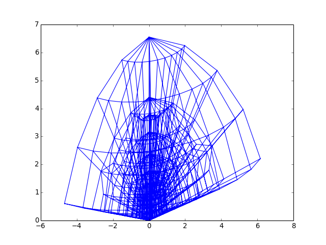
Indenter	half_angle	sweep_angle
Berkovich	65.03	60.00
Modified Berkovich	65.27	60.00
Cube Corner	35.26	60.00
Vickers	68.00	45.00

from abapy.indentation import DeformableCone3D
from matplotlib import pyplot as plt
c = DeformableCone3D(Na =4, Nb = 4, Ns = 1, N = 10, sweep_angle = 120.)
c.make_mesh()
f = open('DeformableCone3D.vtk', 'w')
f.write(c.mesh.dump2vtk())
f.close()
x,y,z = c.mesh.get_edges()
# Adding some 3D "home made" perspective:
zx, zy = .3, .3
for i in xrange(len(x)):
  if x[i] != None:
    x[i] += zx * z[i]
    y[i] += zy * z[i]
plt.plot(x,y)
plt.show()

(Source code, png, hires.png, pdf)

apply_displacement(disp)[source]¶

Applies a displacement field to the indenter.

Parameters:	disp (`abapy.postproc.VectorFieldOutput` instance.) – displacement field (with only one location).

dump2inp()[source]¶

Dumps to Abaqus INP format.

Return type:	string

equivalent_half_angle()[source]¶: Returns the half angle (in degrees) of the equivalent cone in terms of cross area and volume. :retype: float

get_border()[source]¶

Returns a plotable version of the border of the indenter usable directly in matplotlib.pyplot.

Return type:	x and y lists

get_edges()[source]¶

Returns a plotable version of the indenter usable directly in matplotlib.pyplot.

Return type:	x and y lists

set_N(N)[source]¶

Sets the number of sweeped elements

Parameters:	N (int > 1) – N

set_Na(Na)[source]¶

Sets the Na parameter of the indenter (see IndentationMesh for explanations).

Parameters:	Na (int > 1) – Na

set_Nb(Nb)[source]¶

Sets the Nb parameter of the indenter (see IndentationMesh for explanations).

Parameters:	Nb (int > 1) – Nb

set_Nf(Nf)[source]¶

Sets the Nf parameter of the indenter (see IndentationMesh for explanations).

Parameters:	Nf (int > 1) – Nf

set_Ns(Ns)[source]¶

Sets the Ns parameter of the indenter (see `IndentationMesh for explanations).

Parameters:	Ns (int > 1) – Ns

set_half_angle(half_angle=70.3)[source]¶

Sets the half angle of the indenter. Default is equivalent to modified Berkovich indenter in volume.

Parameters:	half_angle (float > 0.) – half_angle in DEGREES.

set_l(l)[source]¶

Sets the l parameter of the indenter (see ParamInfiniteMesh for explanations)

Parameters:	l (float > 0.) – l

set_mat_label(mat_label)[source]¶

Sets the label of the constitutive material of the indenter.

Parameters:	mat_label (string) – mat_label

set_pyramid(pyramid)[source]¶

Sets the indenter as a revolution cone (False) or a pyramid (True). I the case of the pyramid, the half angle becomes the axis to face angle.

Parameters:	pyramid (bool) – True for pyramid, False for revolution (default).

set_rigid(rigid)[source]¶

Sets the indenter to be rigid (True) or deformable (False).

Parameters:	rigid (bool) – True for rigid, False for deformable (default)

set_summit_position(summit_position)[source]¶

Sets the position of the indenter.

Parameters:	summit_position (tuple or list containing two floats.) – position of the summit in a 2D space.

set_sweep_angle(sweep_angle)[source]¶

Sets the sweep angle.

Parameters:	sweep_angle (int > 1) – sweep_angle

Indenter miscellaneous¶

abapy.indentation.equivalent_half_angle(half_angle, sweep_angle)[source]¶: Returns the half angle (in degrees) of the equivalent cone in terms of cross area and volume of a pyramidal indenter. :param half_angle: indenter half angle in degrees :type half_angle: float :param sweep_angle: sweep angle in degrees :type sweep_angle: float :rtype: float

Simulation tools¶

Steps definition¶

class abapy.indentation.Step(name, disp=1.0, nlgeom=True, nframes=100, fieldOutputFreq=999999, boundaries_3D=False, full_3D=False, rigid_indenter_3D=True, nodeFieldOutput=['COORD', 'U'], elemFieldOutput=['LE', 'EE', 'PE', 'PEEQ', 'S'], mode='bulk')[source]¶

Builds a typical indentation step.

Parameters:

name (string) – step name.
disp (float > 0.) – displacement.
nframes (int) – frame number.
nlgeom (boolean) – nlgeom state.
fieldOutputFreq (int) – field output frequency
boundaries_3D (boolean) – 3D or 2D boundary conditions. If 3D is True, then boundary conditions will be applied to the node sets front and back.
full_3D (boolean) – set to True if the model is a complete 3D model without symmetries and then does not need side boundaries.
rigid_indenter_3D (boolean) – Set to True if a 3D indenter is rigid
nodeFieldOutput (string or list of strings) – node outputs.
elemFieldOutput (string or list of strings) – node outputs.

Step.set_name(name)[source]¶

Sets step name.

Parameters:	name (string) – step name.

Step.set_displacement(disp)[source]¶

Sets the displacement.

Parameters:	disp (float > 0.) – displacement.

Step.set_nframes(nframes)[source]¶

Sets the number of frames.

Parameters:	nframes (int) – frame number.

Step.set_nlgeom(nlgeom)[source]¶

Sets NLGEOM on or off.

Parameters:	nlgeom (boolean) – nlgeom state.

Step.set_fieldOutputFreq(freq)[source]¶

Sets the field output period.

Parameters:	freq (int) – field output frequency

Step.set_nodeFieldOutput(nodeOutput)[source]¶

Sets the node field output to be recorded.

Parameters:	nodeOutput (string or list of strings) – node outputs.

Step.set_elemFieldOutput(elemOutput)[source]¶

Sets the element field output to be recorded.

Parameters:	elemOutput (string or list of strings) – node outputs.

Step.dump2inp()[source]¶: Dumps the step to Abaqus INP format.

Inp builder¶

abapy.indentation.MakeInp(sample_mesh=None, indenter=None, sample_mat=None, indenter_mat=None, friction=0.0, steps=None, is_3D=False, heading='Abapy Indentation Simulation')[source]¶

Builds a complete indentation INP for Abaqus and returns it as a string.

Parameters:

sample_mesh (abapy.mesh.Mesh instance or None) – mesh to use for the sample. If None, default ParamInfiniteMesh will be used.
indenter (any indenter instance or None) – indenter to use. If None, default RigidCone2D will be used.
sample_mat (any material instance or None) – sample material to use. If None, default abapy.materials.VonMises will be used.
indenter_mat (any material instance or None) – indenter material to use. If None, a default elastic material will be used. If a rigid indenter is chosen, this material will not interfer with the simulation results.
friction (float >= 0.) – friction coefficient between indenter and sample.
steps (list of Step instances or None) – steps to used during the test.

Return type:

string

#-----------------------
# PACKAGES
from abapy.indentation import MakeInp, DeformableCone2D, DeformableCone3D, IndentationMesh, Step
from abapy.materials import Elastic, VonMises
from math import radians, tan
#-----------------------

#-----------------------
# FIRST EXEMPLE: AXISYMMETRIC INDENTATION
# Model parameters
half_angle = 70.29      # Indenter half angle, 70.3 degrees is equivalent to Berkovich indenter
Na, Nb, Ns, Nf, l = 8, 8, 16, 2, 1.
E, nu = 1., 0.3         # E is the Young's modulus and nu is the Poisson's ratio. 
ey = 0.01 * E
max_disp = l/3.*tan(radians(70.3))/tan(radians(half_angle)) # Maximum displacement

# Building model 
indenter = DeformableCone2D(half_angle = half_angle, rigid = True, Na = Na, Nb = Nb, Ns = Ns, Nf = Nf, l=l) # Indenter
sample_mesh = IndentationMesh(Na = Na, Nb = Nb, Ns = Ns, Nf = Nf, l=l)# Sample Mesh
#sample_mat = Elastic(labels = 'SAMPLE_MAT', E = E, nu=  nu)    # Sample material
sample_mat = VonMises(labels = 'SAMPLE_MAT', E = E, nu=  nu, sy = E * ey)    # Sample material
indenter_mat = Elastic(labels = 'INDENTER_MAT')    # Indenter material
steps = [                                                 # Steps
  Step(name='preloading', nframes = 50, disp = max_disp / 2.),
  Step(name='loading',    nframes = 50, disp = max_disp ), 
  Step(name='unloading',  nframes = 50, disp = 0.), ] 

# Making INP file
inp = MakeInp(indenter = indenter,
sample_mesh = sample_mesh,
sample_mat = sample_mat,
indenter_mat = indenter_mat,
steps = steps)
f = open('workdir/indentation_axi.inp', 'w')
f.write(inp)
f.close() 
#-----------------------

#-----------------------
# SECOND EXAMPLE: 3D BERKOVICH INDENTATION
# Model Parameters
half_angle = 65.27     # Indenter half angle, 65.27 leads to a modified Berkovich geometry, see help(DeformableCone3D for further information)
Na, Nb, Ns, Nf, l = 8, 8, 8, 2, 1. # with 4, 4, 4, 2, 1., simulation is very fast, the mesh is coarse (even crappy) but the result is surprisingly good! 
sweep_angle, N = 60., 8
E, nu = 1., 0.3         # E is the Young's modulus and nu is the Poisson's ratio. 
ey = 0.01 # yield strain
max_disp = l/3.*tan(radians(70.3))/tan(radians(half_angle)) # Maximum displacement
pyramid = True

# Building model
indenter = DeformableCone3D(half_angle = half_angle, rigid = True, Na = Na, Nb = Nb, Ns = Ns, Nf = Nf, N= N, sweep_angle=sweep_angle, l=l, pyramid = pyramid) # Indenter
sample_mesh = IndentationMesh(Na = Na, Nb = Nb, Ns = Ns, Nf = Nf, l=l).sweep(sweep_angle = sweep_angle, N = N)   # Sample Mesh
#sample_mat = Elastic(labels = 'SAMPLE_MAT', E = E, nu=  nu)    # Sample material
sample_mat = VonMises(labels = 'SAMPLE_MAT', E = E, nu=  nu, sy = E * ey)    # Sample material
indenter_mat = Elastic(labels = 'INDENTER_MAT')    # Indenter material
steps = [                                                 # Steps
  Step(name='preloading',   nframes = 100, disp = max_disp / 2., boundaries_3D=True), 
  Step(name='loading',      nframes = 100, disp = max_disp,      boundaries_3D=True), 
  Step(name='unloading',    nframes = 200, disp = 0.,            boundaries_3D=True)] 

# Making INP file.
inp = MakeInp(indenter = indenter,
sample_mesh = sample_mesh,
sample_mat = sample_mat,
indenter_mat = indenter_mat,
steps = steps, is_3D = True)
f = open('workdir/indentation_berko.inp', 'w')
f.write(inp)
f.close() 
#-----------------------

# Simulation can be launched using abaqus job=indentation and can be roughly post processed using abaqus viewer of more finely using abapy.

Returns:

indentation_axi.inp

indentation_berko.inp

Simulation manager¶

class abapy.indentation.Manager(workdir='', abqlauncher='abaqus', samplemesh=None, indenter=None, samplemat=None, indentermat=None, friction=0.0, steps=None, is_3D=False, simname='indentation', files2delete=['sta', 'sim', 'prt', 'odb', 'msg', 'log', 'dat', 'com', 'inp', 'lck', 'pckl'], abqpostproc='abqpostproc.py')[source]¶

The spirit of the simulation manager is to allow you to work at a higher level. Using it allows you to define once and for all where you work, where Abaqus is, it fill manage subprocesses (Abaqus, Abaqus python) automatically. It is particularly interresting to perform parametric simulation because you can modify one parameter (material property, inenter property, ...) and keep all other parameters fixed and rerun directly the simulation process without making any mistake.

Note

This class is still under developpement, important changes may then happen.

Parameters:

workdir (string) – work directory where simulation is to be run.
abqlauncher (string) – abaqus launcher or path to it. Take care about aliases under linux because they often don’t work under non interactive shells. A direct path to the launcher may be a good idea.
samplemesh (abapy.mesh.Mesh instance or None) – mesh to be used by MakeInp, None will let MakeInp use it’s own default.
indenter (indenter instance or None) – indenter to be used by MakeInp, None will let MakeInp use it’s own default.
samplemat (material instance or None) – sample material to be used by MakeInp, None will let MakeInp use it’s own default.
indentermat (material instance or None) – indenter material to be used by MakeInp, None will let MakeInp use it’s own default.
steps (list of Step instances.) – steps to use during the test.
is_3D (Bool) – has to be True if the simulation is 3D, else must be False.
simname (string) – simulation name used for all files.
files2delete (list of strings.) – file types to delete when cleaning work directory.

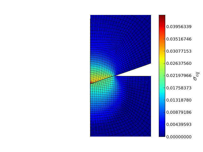
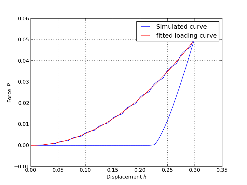
from abapy.indentation import Manager, IndentationMesh, Step, RigidCone2D, DeformableCone2D
from abapy.materials import VonMises, Elastic
from math import radians, tan
import numpy as np
import matplotlib.pyplot as plt
#---------------------------------------
# Python post processing function:
# Role: data extraction from odb is performed in Abaqus python but nothing more. A regular Python version featuring numpy/scipy and matplotlib is so much better to perform custom post processing. That's why we do it in two steps: what cannot be done out of abaqus is done in abaqus, everything else is performed outside.
def pypostproc(data):
  if data['completed']:
    return data
  else: 
    print '<Warning: Simulation aborted, check .msg file for explanations.>'
    return data
#---------------------------------------    
# Defining test parameters:
Na, Nb, Ns, Nf = 16,16, 16, 2
half_angle = 70.29
rigid_indenter = False # Sets the indenter rigid of deformable
mesh = IndentationMesh(Na = Na, Nb = Nb, Ns = Ns, Nf = Nf)                # Chosing sample mesh
#indenter = RigidCone2D(half_angle = 70.3)                 # Chosing indenter
indenter = DeformableCone2D(half_angle = half_angle, Na = Na, Nb = Nb, Ns=Ns, Nf=Nf, rigid = rigid_indenter)  
E = 1.                                                    # Young's modulus
sy = E * .01                                              # Yield stress
samplemat = VonMises(labels = 'SAMPLE_MAT', E = E, sy = sy)   # Sample material
indentermat = Elastic(labels = 'INDENTER_MAT', E = E) 
max_disp = .3 * tan(radians(70.3))/tan(radians(half_angle))
nframes = 200
steps = [                                                 # Steps
  Step(name='loading0', nframes = nframes, disp = max_disp/2.),
  Step(name='loading1', nframes = nframes, disp = max_disp), 
  Step(name = 'unloading', nframes = nframes, disp = 0.)] 
#---------------------------------------
# Directories: absolute pathes seems more secure to me since we are running some 'rm'. 
workdir = 'workdir/'
abqlauncher = '/opt/Abaqus/6.9/Commands/abaqus'
simname = 'indentation'
abqpostproc = 'abqpostproc.py'
#---------------------------------------
# Setting simulation manager
m = Manager()
m.set_abqlauncher(abqlauncher)
m.set_workdir(workdir)
m.set_simname(simname)
m.set_abqpostproc(abqpostproc)
m.set_samplemesh(mesh)
m.set_samplemat(samplemat)
m.set_indentermat(indentermat)
m.set_steps(steps)
m.set_indenter(indenter)
m.set_pypostprocfunc(pypostproc)
#---------------------------------------
# Running simulation and post processing
#m.erase_files() # Workdir cleaning
m.make_inp() # INP creation
#m.run_sim() # Running the simulation
#m.run_abqpostproc() # First round of post processing in Abaqus
data = m.run_pypostproc() # Second round of custom post processing in regular Python

#---------------------------------------

if data['completed']:
  # Ploting results
  step2plot = 0
  Nlevels = 200
  plt.figure(0)
  # Ploting load vs. disp curve
  plt.clf()
  ho = data['history']
  F = -ho['force']
  h = -ho['disp']
  C = (F[1]/h[1]**2).average()
  F_fit = C * h **2
  plt.plot(h.plotable()[1], F.plotable()[1], 'b-',label = 'Simulated curve', linewidth = 1.)
  plt.plot(h[0,1].plotable()[1], F_fit[0,1].plotable()[1],'r-', label = 'fitted loading curve', linewidth = 1.)
  plt.xlabel('Displacement $h$')
  plt.ylabel('Force $P$')
  plt.legend()
  plt.grid()
  plt.savefig(workdir + simname + '_load-disp.png')
  # Ploting deformed shape
  
  plt.clf()
  plt.gca().set_aspect('equal')
  plt.axis('off')
  fo = data['field']
  #stress = fo['S'][step2plot].vonmises()
  stress = fo['S'][step2plot].pressure()
  if 'Sind' in fo.keys():
    #ind_stress = fo['Sind'][step2plot].vonmises()
    ind_stress = fo['Sind'][step2plot].pressure()
  smax= max( max(stress.data), max(ind_stress.data))
  smin= min( min(stress.data), min(ind_stress.data)) 
  #levels = [(n+1)/float(Nlevels)*smax for n in xrange(Nlevels)]  
  levels = np.linspace(smin, smax, Nlevels)
  field_flag = r'$\sigma_{eq}$'
  disp = fo['U'][step2plot]
  ind_disp = fo['Uind'][step2plot]
  indenter.apply_displacement(ind_disp) # Applies the displacement to the indenter.
  
  #plt.plot(xbi,ybi,'k-')
  mesh.nodes.apply_displacement(disp) # This Nodes class method allows to deform a Nodes instance (and the Mesh instance it's nested in by the way) using a VectorFieldOutput. This allows very easy mesh tuning and deformed shape ploting.
  xlim, ylim, zlim = mesh.nodes.boundingBox() # This little method allows nicer ploting producing a bounding box with a little gap around the mesh. This avoids the very tight boxes pyplot tends to use which cut thick lines on the border of the mesh.
  xmin, xmax = 0., 2.
  ymin, ymax = -2., 2.
  plt.xlim([xmin, xmax])
  plt.ylim([ymin, ymax])
  x, y, z, tri = mesh.dump2triplot() # This method translates the whole mesh in matplotlib.pyplot.triplot syntax: x coords, y coords, (z coords useless here but can be nice for perspective effects) and label less connectivity.
  xi, yi, zi, trii = indenter.mesh.dump2triplot()
  xe, ye, ze = mesh.get_edges(xmin = xmin, xmax = xmax, ymin = ymin, ymax = ymax)
  xb, yb, zb = mesh.get_border(xmin = xmin, xmax = xmax, ymin = ymin, ymax = ymax)
  xei, yei, zei = indenter.mesh.get_edges(xmin = xmin, xmax = xmax, ymin = ymin, ymax = ymax) # Gives us a wireframe indenter representation.
  xbi, ybi, zbi = indenter.mesh.get_border(xmin = xmin, xmax = xmax, ymin = ymin, ymax = ymax) # Gives us the border of the indenter.
  plt.plot(xe,ye,'-k', linewidth = 0.5) # Mesh ploting.
  plt.plot(xb,yb,'-k', linewidth = 1.) # Sample border ploting.
  plt.plot(xei,yei,'-k', linewidth = 0.5) # Mesh ploting.
  plt.plot(xbi,ybi,'-k', linewidth = 1.) # Sample border ploting.
  grad = plt.tricontourf(x, y, tri, stress.data, levels) # Gradiant plot, Nlevels specifies the number of levels.
  plt.tricontourf(xi,yi,trii, ind_stress.data, levels)
  #plt.tricontour(xi,yi,trii, ind_stress.data, levels,  colors = 'black')
  cbar = plt.colorbar(grad)
  cbar.ax.set_ylabel(field_flag, fontsize=20)
  #plt.tricontour(x, y, tri, stress.data, levels,  colors = 'black') # Isovalue plot which make gradiant plot clearer in my (humble) opinion.
  #plt.show()
  plt.savefig(workdir + simname + '_field.png')

Gives:

Note

In order to used abaqus Python, you have to build a post processing script that is executed in abaqus python. Here is an example abqpostproc.py:

# ABQPOSTPROC.PY
# Warning: executable only in abaqus abaqus viewer -noGUI,... not regular python.
import sys
from abapy.postproc import GetFieldOutput_byRpt as gfo
from abapy.postproc import GetVectorFieldOutput_byRpt as gvfo
from abapy.postproc import GetTensorFieldOutput_byRpt as gtfo
from abapy.postproc import GetHistoryOutputByKey as gho
from abapy.indentation import Get_ContactData
from abapy.misc import dump
from odbAccess import openOdb
from abaqusConstants import JOB_STATUS_COMPLETED_SUCCESSFULLY



# Odb opening  
file_name = 'indentation'
odb = openOdb(file_name + '.odb')
data = {}

# Check job status:
job_status = odb.diagnosticData.jobStatus

if job_status == JOB_STATUS_COMPLETED_SUCCESSFULLY:
  data['completed'] = True 
  # Field Outputs
  data['field'] = {}
  fo = data['field']
  fo['Uind'] = [
    gvfo(odb = odb, 
      instance = 'I_INDENTER', 
      step = 1,
      frame = -1,
      original_position = 'NODAL', 
      new_position = 'NODAL', 
      position = 'node',
      field = 'U', 
      delete_report = True),
    gvfo(odb = odb, 
      instance = 'I_INDENTER', 
      step = 2,
      frame = -1,
      original_position = 'NODAL', 
      new_position = 'NODAL', 
      position = 'node',
      field = 'U', 
      delete_report = True)]
  
  fo['U'] = [
    gvfo(odb = odb, 
      instance = 'I_SAMPLE', 
      step = 1,
      frame = -1,
      original_position = 'NODAL', 
      new_position = 'NODAL', 
      position = 'node',
      field = 'U', 
      sub_set_type = 'element', 
      delete_report = True),
    gvfo(odb = odb, 
      instance = 'I_SAMPLE', 
      step = 2,
      frame = -1,
      original_position = 'NODAL', 
      new_position = 'NODAL', 
      position = 'node',
      field = 'U', 
      sub_set_type = 'element', 
      delete_report = True)]
      
  fo['S'] = [
    gtfo(odb = odb, 
      instance = 'I_SAMPLE', 
      step = 1,
      frame = -1,
      original_position = 'INTEGRATION_POINT', 
      new_position = 'NODAL', 
      position = 'node',
      field = 'S', 
      sub_set_type = 'element', 
      delete_report = True),
    gtfo(odb = odb, 
      instance = 'I_SAMPLE', 
      step = 2,
      frame = -1,
      original_position = 'INTEGRATION_POINT', 
      new_position = 'NODAL', 
      position = 'node',
      field = 'S', 
      delete_report = True)]
  
  fo['Sind'] = [
    gtfo(odb = odb, 
      instance = 'I_INDENTER', 
      step = 1,
      frame = -1,
      original_position = 'INTEGRATION_POINT', 
      new_position = 'NODAL', 
      position = 'node',
      field = 'S', 
      sub_set_type = 'element', 
      delete_report = True),
    gtfo(odb = odb, 
      instance = 'I_SAMPLE', 
      step = 2,
      frame = -1,
      original_position = 'INTEGRATION_POINT', 
      new_position = 'NODAL', 
      position = 'node',
      field = 'S', 
      delete_report = True)]
       
  fo['LE'] = [
    gtfo(odb = odb, 
      instance = 'I_SAMPLE', 
      step = 1,
      frame = -1,
      original_position = 'INTEGRATION_POINT', 
      new_position = 'NODAL', 
      position = 'node',
      field = 'LE', 
      sub_set_type = 'element', 
      delete_report = True),
    gtfo(odb = odb, 
      instance = 'I_SAMPLE', 
      step = 2,
      frame = -1,
      original_position = 'INTEGRATION_POINT', 
      new_position = 'NODAL', 
      position = 'node',
      field = 'LE', 
      sub_set_type = 'element', 
      delete_report = True)] 
      
  fo['EE'] = [
    gtfo(odb = odb, 
      instance = 'I_SAMPLE', 
      step = 1,
      frame = -1,
      original_position = 'INTEGRATION_POINT', 
      new_position = 'NODAL', 
      position = 'node',
      field = 'EE', 
      sub_set_type = 'element', 
      delete_report = True),
    gtfo(odb = odb, 
      instance = 'I_SAMPLE', 
      step = 2,
      frame = -1,
      original_position = 'INTEGRATION_POINT', 
      new_position = 'NODAL', 
      position = 'node',
      field = 'EE', 
      sub_set_type = 'element', 
      delete_report = True)]     
  
  fo['PE'] = [
    gtfo(odb = odb, 
      instance = 'I_SAMPLE', 
      step = 1,
      frame = -1,
      original_position = 'INTEGRATION_POINT', 
      new_position = 'NODAL', 
      position = 'node',
      field = 'PE', 
      sub_set_type = 'element', 
      delete_report = True),
    gtfo(odb = odb, 
      instance = 'I_SAMPLE', 
      step = 2,
      frame = -1,
      original_position = 'INTEGRATION_POINT', 
      new_position = 'NODAL', 
      position = 'node',
      field = 'PE', 
      sub_set_type = 'element', 
      delete_report = True)] 
  
  fo['PEEQ'] = [
    gfo(odb = odb, 
      instance = 'I_SAMPLE', 
      step = 1,
      frame = -1,
      original_position = 'INTEGRATION_POINT', 
      new_position = 'NODAL', 
      position = 'node',
      field = 'PEEQ', 
      sub_set_type = 'element', 
      delete_report = True),
    gfo(odb = odb, 
      instance = 'I_SAMPLE', 
      step = 2,
      frame = -1,
      original_position = 'INTEGRATION_POINT', 
      new_position = 'NODAL', 
      position = 'node',
      field = 'PEEQ', 
      sub_set_type = 'element', 
      delete_report = True)] 
  # History Outputs
  data['history'] = {} 
  ho = data['history']
  ref_node = odb.rootAssembly.instances['I_INDENTER'].nodeSets['REF_NODE'].nodes[0].label
  ho['force'] =  gho(odb,'RF2')['Node I_INDENTER.'+str(ref_node)] # GetFieldOutputByKey returns all the occurences of the required output (here 'RF2') and stores it in a dict. Each dict key refers to a location. Here we have to specify the location ('Node I_INDENTER.1') mainly for displacement which has been requested at several locations.
  ho['disp'] =   gho(odb,'U2')['Node I_INDENTER.'+str(ref_node)]
  tip_node = odb.rootAssembly.instances['I_INDENTER'].nodeSets['TIP_NODE'].nodes[0].label
  ho['tip_penetration'] =   gho(odb,'U2')['Node I_INDENTER.'+str(tip_node)]
  ho['allse'] =   gho(odb,'ALLSE').values()[0]
  ho['allpd'] =   gho(odb,'ALLPD').values()[0]
  ho['allfd'] =   gho(odb,'ALLFD').values()[0]
  ho['allwk'] =   gho(odb,'ALLWK').values()[0]
  #ho['carea'] =  gho(odb,'CAREA    ASSEMBLY_I_SAMPLE_SURFACE_FACES/ASSEMBLY_I_INDENTER_SURFACE_FACES').values()[0]
  
  # CONTACT DATA PROCESSING
  ho['contact'] = Get_ContactData(odb = odb, instance = 'I_SAMPLE', node_set = 'TOP_NODES')
 
else:
  data['completed'] = False
# Closing and dumping
odb.close()
dump(data, file_name+'.pckl')

Settings¶

Manager.set_simname(simname)[source]¶

Sets simname.

Parameters:	simname (string) – simulation name that is used to name simulation files.

Manager.set_workdir(workdir)[source]¶

Sets work directory

Parameters:	workdir (string) – relative or absolute path to workdir where simulations are run.

Manager.set_abqlauncher(abqlauncher)[source]¶: Sets Abaqus launcher :param abqlauncher: alias, relative path or absolute path to abaqus launcher. :type abqlaucher: string

Manager.set_samplemesh(samplemesh)[source]¶

Sets sample mesh.

Parameters:	samplemesh (`abapy.mesh.Mesh` instance) – sample mesh.

Manager.set_indenter(indenter)[source]¶

Sets indenter.

Parameters:	indenter (instance of any indenter class) – indenter to be used.

Manager.set_samplemat(samplemat)[source]¶

Sets sample material.

Parameters:	samplemat (instance of any material class) – core material.

Manager.set_steps(steps)[source]¶

Sets steps

Parameters:	steps (list `of Steps` instances) – description of steps.

Manager.set_files2delete(files2delete)[source]¶

Sets files to delete when cleaning.

Parameters:	files2delete (list of strings.) – files types to be deleted when cleaning workdir.

Manager.set_abqpostproc(abqpostproc)[source]¶

Sets the path to the abaqus post-processing python script, this path must be absolute or relative to workdir.

Parameters:	abqpostproc (string) – link to the abaqus post processing script.

Manager.set_pypostprocfunc(func)[source]¶

Sets the Python post processing function.

Parameters:	func (function) – post processing function of the data produced by abaqus post processing.

Launchers¶

Manager.erase_files()[source]¶: Erases all files with types declared in files2delete in the work directory with the name simname.

Manager.make_inp()[source]¶: Builds the INP file using MakeInp and stores it in workdir as “simname.inp”.

Manager.run_sim()[source]¶: Runs the simulation.

Manager.run_abqpostproc()[source]¶: Runs the first pass of post processing inside Abaqus Python.

Manager.run_pypostproc()[source]¶

Runs the Python post processing function.

Return type:	data returned by pypostprocfunc

Indentation post-processing¶

Contact Data¶

class abapy.indentation.ContactData(repeat=3, is_3D=False, dtf='f')[source]¶

ContactData class aims to store and proceed all contact related data:

Position of nodes involved in the contact relationship.

Contact pressure on these nodes.

This class can be used to perform various tasks:

Find contact shape.

Compute contact area.

Find contact contour.

Produce matrix (AFM-like) images using the SPYM module.

Parameters:

repeat (int > 0) – this parameter is only used in the case of 3D contact. Due to symmetries, only a portion of the problem is computed. To get back to complete problem, a symmetry has to be performed and then a given number of copies of the result, this number is repeat. For example, to simulate a Vickers 4 sided indenter indentation, you will compute only 1 / 8 of the problem. So after a symmetry, you will need 4 copies of the result, the repeat = 4. To summarize, repeat is the number of faces of the indenter.
is_3D (bool) – True for 3D contact, False for axisymmetric contact.
dtf (string) – array.array data type for floats, ‘f’ for 32 bit float, ‘d’ for 64 float.

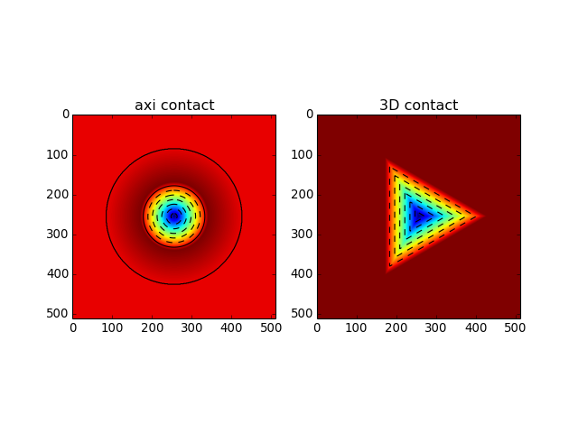
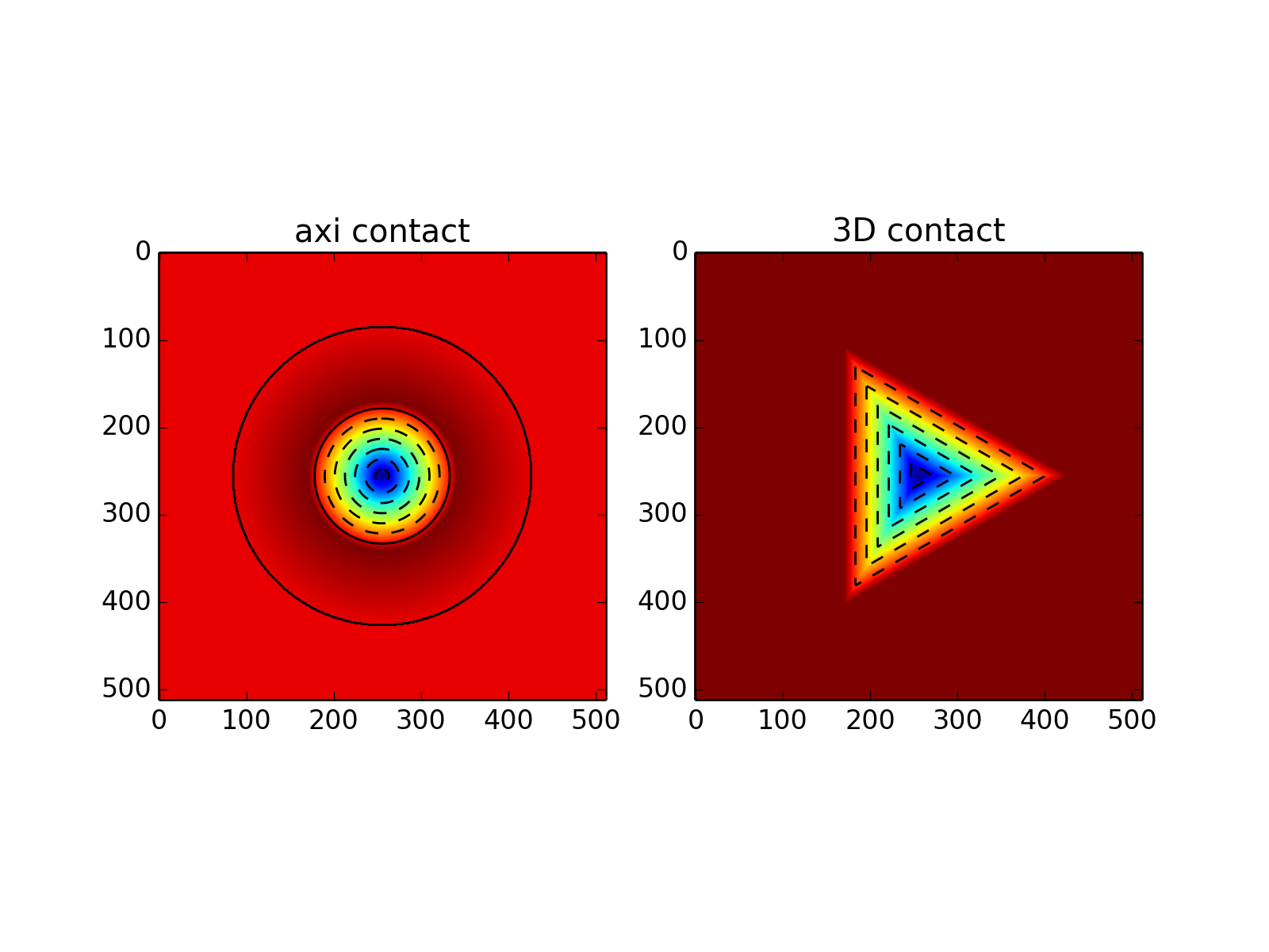
import numpy as np
from abapy.indentation import ContactData

X = np.linspace(-3., 3., 512)
Y = np.linspace(-3., 3., 512)
X, Y = np.meshgrid(X, Y)
# Axi
cd = ContactData()
x = [0, 1, 2, 10]
alt = [-1,.1, 0, 0]
press = [1, 0, 0, 0]
cd.add_data(x, altitude = alt, pressure = press)
Alt_axi, Press_axi = cd.interpolate(X, Y, method ='linear')
area = cd.contact_area()


# 3D
cd = ContactData(repeat = 3, is_3D = True)
k = np.cos(np.radians(60))
p = np.sin(np.radians(60))
x = [0, 4, 10, k*4, k*10]
y = [0, 0, 0,  p*4, p*10]
alt = [-1, 0, 0, 0, 0]
cd.add_data(x, altitude = alt)
Alt_3D, Press_3D = cd.interpolate(X, Y, method ='linear')


from matplotlib import pyplot as plt

fig = plt.figure()
plt.clf()
ax1 = fig.add_subplot(121)
grad = plt.imshow(Alt_axi)
plt.contour(Alt_axi, colors= 'black')
plt.title('axi contact')
ax1 = fig.add_subplot(122)
grad = plt.imshow(Alt_3D)
plt.contour(Alt_3D, colors= 'black')
plt.title('3D contact')
plt.show()

(Source code, png, hires.png, pdf)

add_data(coor1, coor2=0.0, altitude=0.0, pressure=0.0)[source]¶

Adds data to a ContactData instance.

Parameters:	coor1 (float or list like) – radial position in the axisymmetric case or in plane position first coordinate in the 3D case. coor2 (float of list like) – orthoradial position in the axisymmetric case of second in plane coordinate in the 3D case. altitude (float or list like) – out of plane position. pressure (float or list like) – normal contact pressure.

contact_area(delaunay_disp=None)[source]¶: Returns the cross area of contact using the contact pressure field. The contact area is computed using a Delaunay triangulation of the available data points. This triangulation can be oriented using the delaunay_disp option (use very carefuly).

contact_contour(delaunay_disp=None)[source]¶: Returns the contour of the contact zone.

export2spym(lx, ly, xc=0.0, yc=0.0, nx=256, ny=256, xy_unit='m', alt_unit='m', press_unit='Pa', axi_repeat=100, delaunay_disp=None, method='linear')[source]¶

Exports data to spym.generic.Spm_image format.

Parameters:	lx (float) – length on x axis ly (float) – length on y axis xc (float) – position of the center of the image on the x axis yc (float) – position of the center of the image on the y axis nx (uint) – x resolution ny (uint) – y resolution xy_unit (str) – xy unit alt_unit (str) – altitude unit press_unit (str) – contact pressure unit

See get_3D_data for other params.

from abapy.misc import load
import numpy as np
import matplotlib.pyplot as plt

# In this case, a 3D FEM simulation has beed performed and the results are stored in the file ``ContactData.pckl``. See ``Get_ContactData`` to understand how this data has been extracted from an Abaqus odb file.


out = load('ContactData_berk.pckl')
cdl = out[1][-1] # loading
cdu = out[2][-1] # unloading
hmax = -cdl.min_altitude()
l = 7. * hmax
alt, press = cdu.export2spym(lx = l, ly = l, nx = 512, ny = 512)
alt.dump2gsf('image.gsf')
xlabel, ylabel, zlabel = alt.get_labels()
X,Y,Z = alt.get_xyz()
plt.figure()
plt.clf()
plt.gca().set_aspect('equal')
plt.grid()
plt.contourf(X, Y, Z, 10)
cbar = plt.colorbar()
cbar.set_label(zlabel)
plt.contour(X, Y, Z, 10, colors = 'black')
plt.xlabel(xlabel)
plt.ylabel(ylabel)
plt.show()

(Source code, png, hires.png, pdf)

This script also produces a GSF image file, readable by both spym and Gwyddion: image.gsf

get_3D_data(axi_repeat=100, delaunay_disp=None, crit_dist=1e-05)[source]¶

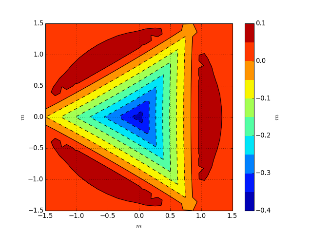
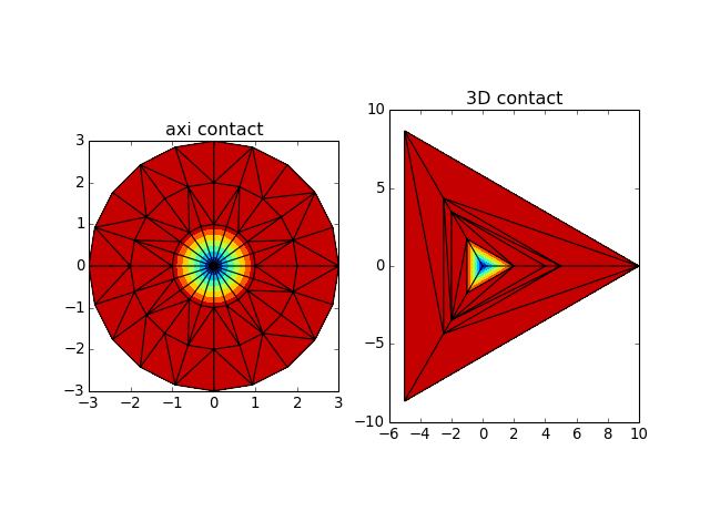
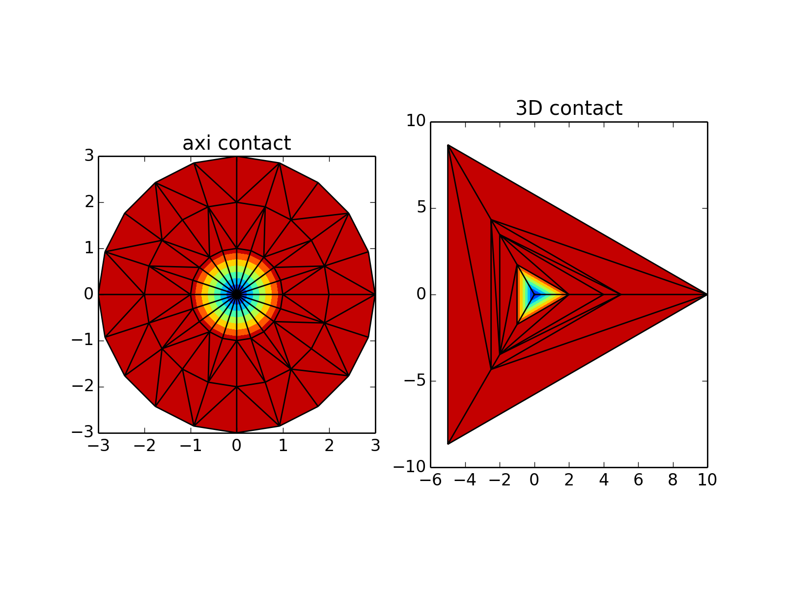
Returns full 3D data usable for interpolation or for ploting. This method performs all the copy and paste needed to get the complete contact (due to symmetries) and also producec a triangular mesh of the surface using the Delaunay algorithm (via scipy).

Parameters:	axi_repeat (int > 0) – number of times axisymmetric profile has to be pasted orthoradially.
Return type:	3 arrays points, alt, press and conn

from abapy.indentation import ContactData
from matplotlib import pyplot as plt


# Axi contact
cd = ContactData()
x = [0, 1, 2, 3]
alt = [-1,.1, 0, 0]
press = [1, 0, 0, 0]
cd.add_data(x, altitude = alt, pressure = press)
points_axi, alt_axi, press_axi, conn_axi = cd.get_3D_data(axi_repeat = 20)



# 3D contact
cd = ContactData(repeat = 3, is_3D = True)
k = np.cos(np.radians(60))
p = np.sin(np.radians(60))
x = [0, 4, 10, k*4, k*10]
y = [0, 0, 0,  p*4, p*10]
alt = [-1, 0, 0, 0, 0]
cd.add_data(x, altitude = alt)
points_3D, alt_3D, press_3D, conn_3D = cd.get_3D_data()



fig = plt.figure()
plt.clf()
ax1 = fig.add_subplot(121)
ax1.set_aspect('equal')
plt.tricontourf(points_axi[:,0], points_axi[:,1], conn_axi, alt_axi)
plt.triplot(points_axi[:,0], points_axi[:,1], conn_axi)

plt.title('axi contact')
ax1 = fig.add_subplot(122)
ax1.set_aspect('equal')
plt.tricontourf(points_3D[:,0], points_3D[:,1], conn_3D, alt_3D)
plt.triplot(points_3D[:,0], points_3D[:,1], conn_3D)
plt.title('3D contact')
plt.show()

(Source code, png, hires.png, pdf)

interpolate(coor1, coor2, axi_repeat=100, delaunay_disp=None, method='linear')[source]¶

Allows general interpolation on the a contact data instance.

Parameters:	coor1 (any list/array of floats) – radial position in the axisymmetric case or in plane position first coordinate in the 3D case. coor2 (any list/array of floats) – orthoradial position in the axisymmetric case of second in plane coordinate in the 3D case. axi_repeat (int > 0) – number of times axisymmetric profile has to be pasted orthoradially.

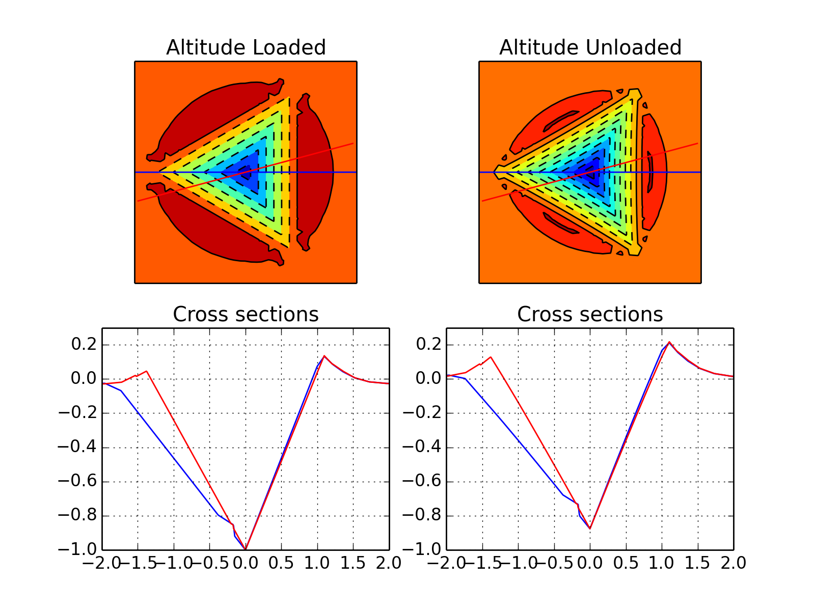
from abapy.misc import load
import numpy as np
from matplotlib import pyplot as plt


# In this case, a 3D FEM simulation has beed performed and the results are stored in the file ``ContactData_berk.pckl``. See ``Get_ContactData`` to understand how this data has been extracted from an Abaqus odb file.


out = load('ContactData_berk.pckl')
cd0 = out[1][-1] # First step data: loading
cd1 = out[2][-1] # Second step data: unloading
hmax = -cd0.min_altitude()

# First let's map altitude and pressure on cartesian grids.
x = np.linspace(-2., 2., 256)
X, Y = np.meshgrid(x, x)

Alt0, Press0 = cd0.interpolate(X, Y, method ='linear')
Alt1, Press1 = cd1.interpolate(X, Y, method ='linear')
Alt0 = Alt0 / hmax
Alt1 = Alt1 / hmax

# Now we wan to get some sections of the imprint
s = np.linspace(0., 2., 256)
s = np.append((-s)[::-1], s)
theta0 = np.radians(0.01)
theta1 = np.radians(15.)
xs0 = np.cos(theta0) * s
ys0 = np.sin(theta0) * s
xs1 = np.cos(theta1) * s
ys1 = np.sin(theta1) * s
# Sections under full load
Alt0_sec_l, Press0_sec_l = cd0.interpolate(xs0, ys0, method ='linear')
Alt1_sec_l, Press1_sec_l = cd0.interpolate(xs1, ys1, method ='linear')
Alt0_sec_l = Alt0_sec_l / hmax
Alt1_sec_l = Alt1_sec_l / hmax
# Sections after unloading
Alt0_sec_u, Press0_sec_u = cd1.interpolate(xs0, ys0, method ='linear')
Alt1_sec_u, Press1_sec_u = cd1.interpolate(xs1, ys1, method ='linear')
Alt0_sec_u = Alt0_sec_u / hmax
Alt1_sec_u = Alt1_sec_u / hmax





fig = plt.figure()
plt.clf()
ax1 = fig.add_subplot(221)
ax1.set_xticks([])
ax1.set_yticks([])
grad = plt.contourf(X, Y, Alt0, 10)
plt.contour(X, Y, Alt0, 10, colors = 'black')
plt.grid()
plt.plot(xs0, ys0, 'b-')
plt.plot(xs1, ys1, 'r-')
ax1.set_aspect('equal')
plt.title('Altitude Loaded')
ax2 = fig.add_subplot(222)
ax2.set_xticks([])
ax2.set_yticks([])
grad = plt.contourf(X, Y, Alt1, 10)
plt.contour(X, Y, Alt1, 10, colors = 'black')
plt.grid()
plt.plot(xs0, ys0, 'b-')
plt.plot(xs1, ys1, 'r-')
ax2.set_aspect('equal')
plt.title('Altitude Unloaded')
ax3 = fig.add_subplot(223)
ax3.set_ylim([-1,0.3])
plt.plot(s, Alt0_sec_l, 'b-')
plt.plot(s, Alt1_sec_l, 'r-')
plt.title('Cross sections')
plt.grid()
ax4 = fig.add_subplot(224)
ax4.set_ylim([-1,0.3])
plt.plot(s, Alt0_sec_u, 'b-')
plt.plot(s, Alt1_sec_u, 'r-')
plt.title('Cross sections')
plt.grid()
plt.show()

(Source code, png, hires.png, pdf)

max_altitude()[source]¶: Returns the maximum altitude.

max_pressure()[source]¶: Returns the maximum pressure.

min_altitude()[source]¶: Returns the minimum altitude.

min_pressure()[source]¶: Returns the minimum pressure.

Get Contact Data¶

abapy.indentation.Get_ContactData(odb, instance, node_set)[source]¶

Finds and reformulate contact data on a given node set and a give instance. This function aims to read in Abaqus odb files and is then only usable in abaqus python and abaqus viewer -noGUI. Following conventions are used:

The normal to the initial surface must be the y axis.
In axisymmetrical simulations, this is nearly automatic. In 3D simulations, the initial plane surface must be in parallel to the (x,z) plane.
As a consequence, coor1 will be x, coor2 will be z and the altitude is y.

Parameters:	odb (odb instance obtained using `odbAccess.openOdb`.) – the odb instance where needed data is. instance (string) – name of an instance in contact. node_set (string) – name of a node set belonging to the instance.

Elasticity¶

Hertz¶

class abapy.indentation.Hertz(F=1.0, a=None, h=None, R=1.0, E=1.0, nu=0.3)[source]¶

Hertz spherical indentation model.

from abapy.indentation import Hertz
from abapy.mesh import Mesh, Nodes, RegularQuadMesh
from matplotlib import pyplot as plt
import numpy as np

"""
===========
Hertz model
===========
"""

H = Hertz(F = 1., E=1., nu = 0.1)
Ne = 50

mesh = RegularQuadMesh(N1 = Ne, N2 = Ne, l1 = H.a * 2., l2 = H.a * 2., dtf = 'd')
mesh.nodes.translate(H.a/20., H.a/20.)
S = mesh.nodes.eval_tensorFunction(H.sigma)
R,Z,T,tri = mesh.dump2triplot()
R, Z = np.array(R), np.array(Z)
# Some fields
srr = S.get_component(11)
szz = S.get_component(22)
stt = S.get_component(33)
srz = S.get_component(12)
smises = S.vonmises()
s1, s2, s3, v1, v2, v3 = S.eigen() # Eigenvalues and eigenvectors
data = smises.data

N = 20
levels = np.linspace(0., max(data), N)
a = H.a
plt.figure()
plt.tricontourf(R/a, Z/a, tri, data, levels)
plt.colorbar()
plt.tricontour(R/a, Z/a, tri, data, levels, colors = 'black')
plt.xlabel('$r/a$', fontsize = 14.)
plt.ylabel('$z/a$', fontsize = 14.)
#plt.quiver(R, Z, v1.data1, v1.data2)
plt.grid()
plt.show()

(Source code)

Eeq¶: Eeq: equivalent modulus (GPa)

get_Eeq()[source]¶: Eeq: equivalent modulus (GPa)

sigma(r, z, t=0.0, labels=None)[source]¶: To do.

Hanson¶

class abapy.indentation.Hanson(F=None, a=None, h=None, half_angle=70.29, E=1.0, nu=0.3)[source]¶

Hanson conical indentation model.

from abapy.indentation import Hanson
from abapy.mesh import Mesh, Nodes, RegularQuadMesh
from matplotlib import pyplot as plt
import numpy as np

"""
===========
Hanson model for conical indentation
===========
"""

H = Hanson(F = 1., E=1., nu = 0.3, half_angle = 70.29)
Ne = 20

mesh = RegularQuadMesh(N1 = Ne, N2 = Ne, l1 = H.a * 2., l2 = H.a * 2., dtf = 'd')
mesh.nodes.translate(H.a/20., H.a/20.)
S = mesh.nodes.eval_tensorFunction(H.sigma)
R,Z,T,tri = mesh.dump2triplot()
R, Z = np.array(R), np.array(Z)
# Some fields
srr = S.get_component(11)
szz = S.get_component(22)
stt = S.get_component(33)
srz = S.get_component(12)
smises = S.vonmises()
s1, s2, s3, v1, v2, v3 = S.eigen() # Eigenvalues and eigenvectors
data = smises.data

N = 20
levels = np.linspace(0., max(data), N)
a = H.a
plt.figure()
plt.tricontourf(R/a, Z/a, tri, data, levels)
plt.colorbar()
plt.tricontour(R/a, Z/a, tri, data, levels, colors = 'black')
plt.xlabel('$r/a$', fontsize = 14.)
plt.ylabel('$z/a$', fontsize = 14.)
#plt.quiver(R, Z, v1.data1, v1.data2)
plt.grid()
plt.show()

(Source code)

Eeq¶: Eeq: equivalent modulus (GPa)

get_Eeq()[source]¶: Eeq: equivalent modulus (GPa)

sigma(r, z, t=0.0, labels=None)[source]¶: To do.

Indentation¶

Indentation meshes¶

ParamInfiniteMesh function¶

IndentationMesh function¶

Indenters¶

RigidCone2D class¶

DeformableCone2D class¶

DeformableCone3D class¶

Indenter miscellaneous¶

Simulation tools¶

Steps definition¶

Inp builder¶

Simulation manager¶

Settings¶

Launchers¶

Indentation post-processing¶

Contact Data¶

Get Contact Data¶

Elasticity¶

Hertz¶

Hanson¶

`ParamInfiniteMesh` function¶

`IndentationMesh` function¶

`RigidCone2D` class¶

`DeformableCone2D` class¶

`DeformableCone3D` class¶